The logistic regression on loan’s report
August, 2019
1 Objective
The goal of this session is trying to fit a Logistic Regression model on Loan data aiming to predict the probability of delinquency for each contract.
2 Modeling
2.1 Dataset preparation
Using the vanilla transaction dataset, we calculated several derived variables for each account as described in the Data Preparation session.
This dataset is joined with Loan, Client, Credit Card, District, Account and Account Balance tables.
We ended up having a data set with 118 variables.
| variables |
|---|
| y_loan_defaulter |
| x_account_balance |
| x_average_salary |
| x_avg_account_balance |
| x_card_age_month |
| x_card_type_classic |
| x_card_type_gold |
| x_card_type_junior |
| x_client_age |
| x_client_gender_male |
| x_district_name_Benesov |
| x_district_name_Beroun |
| x_district_name_Blansko |
| x_district_name_Breclav |
| x_district_name_Brno_mesto |
| x_district_name_Brno_venkov |
| x_district_name_Bruntal |
| x_district_name_Ceska_Lipa |
| x_district_name_Ceske_Budejovice |
| x_district_name_Cesky_Krumlov |
| x_district_name_Cheb |
| x_district_name_Chomutov |
| x_district_name_Chrudim |
| x_district_name_Decin |
| x_district_name_Domazlice |
| x_district_name_Frydek_Mistek |
| x_district_name_Havlickuv_Brod |
| x_district_name_Hl.m._Praha |
| x_district_name_Hodonin |
| x_district_name_Hradec_Kralove |
| x_district_name_Jablonec_n._Nisou |
| x_district_name_Jesenik |
| x_district_name_Jicin |
| x_district_name_Jihlava |
| x_district_name_Jindrichuv_Hradec |
| x_district_name_Karlovy_Vary |
| x_district_name_Karvina |
| x_district_name_Kladno |
| x_district_name_Klatovy |
| x_district_name_Kolin |
| x_district_name_Kromeriz |
| x_district_name_Kutna_Hora |
| x_district_name_Liberec |
| x_district_name_Litomerice |
| x_district_name_Louny |
| x_district_name_Melnik |
| x_district_name_Mlada_Boleslav |
| x_district_name_Most |
| x_district_name_Nachod |
| x_district_name_Novy_Jicin |
| x_district_name_Nymburk |
| x_district_name_Olomouc |
| x_district_name_Opava |
| x_district_name_Ostrava_mesto |
| x_district_name_Pardubice |
| x_district_name_Pelhrimov |
| x_district_name_Pisek |
| x_district_name_Plzen_jih |
| x_district_name_Plzen_mesto |
| x_district_name_Plzen_sever |
| x_district_name_Prachatice |
| x_district_name_Praha_vychod |
| x_district_name_Praha_zapad |
| x_district_name_Prerov |
| x_district_name_Pribram |
| x_district_name_Prostejov |
| x_district_name_Rakovnik |
| x_district_name_Rokycany |
| x_district_name_Rychnov_nad_Kneznou |
| x_district_name_Semily |
| x_district_name_Strakonice |
| x_district_name_Sumperk |
| x_district_name_Svitavy |
| x_district_name_Tabor |
| x_district_name_Tachov |
| x_district_name_Teplice |
| x_district_name_Trebic |
| x_district_name_Trutnov |
| x_district_name_Uherske_Hradiste |
| x_district_name_Usti_nad_Labem |
| x_district_name_Usti_nad_Orlici |
| x_district_name_Vsetin |
| x_district_name_Vyskov |
| x_district_name_Zdar_nad_Sazavou |
| x_district_name_Zlin |
| x_district_name_Znojmo |
| x_last_transaction_age_days |
| x_loan_amount |
| x_loan_duration |
| x_loan_payments |
| x_no_of_cities |
| x_no_of_commited_crimes_1995 |
| x_no_of_commited_crimes_1996 |
| x_no_of_enterpreneurs_per_1000_inhabitants |
| x_no_of_inhabitants |
| x_no_of_municip_2000_to_9999 |
| x_no_of_municip_500_to_1999 |
| x_no_of_municip_greater_10000 |
| x_no_of_municip_inhabitants_less_499 |
| x_prop_household |
| x_prop_insurance_payment |
| x_prop_interest_credited |
| x_prop_loan_payment |
| x_prop_old_age_pension |
| x_prop_other |
| x_prop_statement |
| x_ratio_of_urban_inhabitants |
| x_region_central_Bohemia |
| x_region_east_Bohemia |
| x_region_north_Bohemia |
| x_region_north_Moravia |
| x_region_Prague |
| x_region_south_Bohemia |
| x_region_south_Moravia |
| x_transaction_amount |
| x_transaction_count |
| x_unemploymant_rate_1995 |
| x_unemploymant_rate_1996 |
2.2 Variable selection
Starting from this dataset we investigate the presence of redundant or variables not useful for the model such as the ones with not enough variability or with multicollinearity.
2.2.1 Dummy variables
Starting with the dummy variables. We will keep only dummies that has the event in at least 5% of the observation in the dataset.
The below table shows the dummy variables that will be kept in the model:
dummy_variables <- dplyr::select(loan_dataset_logistic,
                                 starts_with('x_client_gender'),
                                 starts_with('x_district_name'),
                                 starts_with('x_region'),
                                 starts_with('x_card_type'))

dummy_variables_high <- tibble(variables = names(dummy_variables),
       zeros = sapply(dummy_variables,
                      function(x) table(as.character(x) == 0)["TRUE"]),
       ones = sapply(dummy_variables,
                     function(x) table(as.character(x) == 1)["TRUE"])) %>%
  mutate(prop_ones = round(ones / (zeros + ones) * 100, 2)) %>%
  arrange(prop_ones) %>%
  filter(prop_ones  > 5)

kable(dummy_variables_high)| variables | zeros | ones | prop_ones |
|---|---|---|---|
| x_region_south_Bohemia | 621 | 61 | 8.94 |
| x_region_north_Bohemia | 620 | 62 | 9.09 |
| x_district_name_Hl.m._Praha | 603 | 79 | 11.58 |
| x_region_Prague | 603 | 79 | 11.58 |
| x_region_central_Bohemia | 595 | 87 | 12.76 |
| x_region_east_Bohemia | 595 | 87 | 12.76 |
| x_region_north_Moravia | 565 | 117 | 17.16 |
| x_region_south_Moravia | 549 | 133 | 19.50 |
| x_card_type_classic | 549 | 133 | 19.50 |
| x_client_gender_male | 348 | 334 | 48.97 |
The remaining dummies will be excluded from the dataset as they do not have enough variability to fit a logistic model on them.
2.2.2 Transaction type proportion variables
After we investigated the low variability in the dummies, we take care of the calculated variables on the transaction type proportion we calculated during the data enhancement process.
prop_variables <- dplyr::select(loan_dataset_logistic,
                                starts_with('x_prop'))

prop_variables <- summary(prop_variables)

kable(t(prop_variables))| x_prop_household | Min. :0.00000 | 1st Qu.:0.00000 | Median :0.08994 | Mean :0.10975 | 3rd Qu.:0.20138 | Max. :0.37573 |
| x_prop_insurance_payment | Min. :0.00000 | 1st Qu.:0.00000 | Median :0.00000 | Mean :0.02088 | 3rd Qu.:0.00000 | Max. :0.32182 |
| x_prop_interest_credited | Min. :0.02873 | 1st Qu.:0.08951 | Median :0.11634 | Mean :0.13651 | 3rd Qu.:0.16048 | Max. :0.63444 |
| x_prop_loan_payment | Min. :0.0002408 | 1st Qu.:0.0475180 | Median :0.0892142 | Mean :0.0986434 | 3rd Qu.:0.1392529 | Max. :0.3025147 |
| x_prop_old_age_pension | Min. :0 | 1st Qu.:0 | Median :0 | Mean :0 | 3rd Qu.:0 | Max. :0 |
| x_prop_other | Min. :0.1549 | 1st Qu.:0.5096 | Median :0.5962 | Mean :0.5923 | 3rd Qu.:0.6889 | Max. :0.8681 |
| x_prop_statement | Min. :0.0001203 | 1st Qu.:0.0229538 | Median :0.0283864 | Mean :0.0391546 | 3rd Qu.:0.0361376 | Max. :0.1883587 |
The variable x_prop_old_age_pension is also excluded from the dataset as it has not a single observation in this sample.
We ended up having a data set with 40 variables.
| variables |
|---|
| y_loan_defaulter |
| x_account_balance |
| x_average_salary |
| x_avg_account_balance |
| x_card_age_month |
| x_card_type_classic |
| x_client_age |
| x_client_gender_male |
| x_district_name_Hl.m._Praha |
| x_last_transaction_age_days |
| x_loan_amount |
| x_loan_duration |
| x_loan_payments |
| x_no_of_cities |
| x_no_of_commited_crimes_1995 |
| x_no_of_commited_crimes_1996 |
| x_no_of_enterpreneurs_per_1000_inhabitants |
| x_no_of_inhabitants |
| x_no_of_municip_2000_to_9999 |
| x_no_of_municip_500_to_1999 |
| x_no_of_municip_greater_10000 |
| x_no_of_municip_inhabitants_less_499 |
| x_prop_household |
| x_prop_insurance_payment |
| x_prop_interest_credited |
| x_prop_loan_payment |
| x_prop_other |
| x_prop_statement |
| x_ratio_of_urban_inhabitants |
| x_region_central_Bohemia |
| x_region_east_Bohemia |
| x_region_north_Bohemia |
| x_region_north_Moravia |
| x_region_Prague |
| x_region_south_Bohemia |
| x_region_south_Moravia |
| x_transaction_amount |
| x_transaction_count |
| x_unemploymant_rate_1995 |
| x_unemploymant_rate_1996 |
2.2.3 Multicollinearity on feature variables
Multicollinearity is the phenomenon in which a given predictor has a strong correlation with one or more predictors, in this scenario the multiple regression coefficient estimates may vary erratically depending on the data, or the model may not even be possible to be calculate in the case of a perfect correlation on the predictors.
So before we try to fit a model we ran a multicollinearity test to identify additional variables to drop from the model specification.
The idea here is to identify the variables with high correlation among them and keep just the variables that have no strong correlation to the other predictors. We will do so by preferring to keep the variables that have lowest correlation against the others.
Just looking at correlation indexes among pairs of predictors is limited as it is possible that the pairwise correlations are small, and yet a linear dependence exists among three or more variables.
That’s why we will rely on a test called Variance Inflation Factors, VIF for short, to detect multicollinearity.
Multicollinearity is poison for Regression algorithms!!!
vars.quant <- select_if(loan_dataset_logistic, is.numeric)
VIF <- imcdiag(vars.quant, loan_dataset_logistic$y_loan_defaulter)

VIF_Table_Before <- tibble(variable = names(VIF$idiags[,1]),
                    VIF = VIF$idiags[,1]) %>%
             arrange(desc(VIF))

knitr::kable(VIF_Table_Before)| variable | VIF |
|---|---|
| x_district_name_Hl.m._Praha | Inf |
| x_region_Prague | Inf |
| x_no_of_commited_crimes_1996 | 1737.252782 |
| x_no_of_inhabitants | 675.671761 |
| x_prop_other | 158.883814 |
| x_prop_household | 121.322251 |
| x_prop_interest_credited | 63.016856 |
| x_prop_loan_payment | 42.844366 |
| x_prop_insurance_payment | 33.485319 |
| x_unemploymant_rate_1996 | 17.565631 |
| x_average_salary | 14.792865 |
| x_unemploymant_rate_1995 | 13.836322 |
| x_transaction_amount | 13.273428 |
| x_prop_statement | 12.772024 |
| x_transaction_count | 12.427778 |
| x_region_north_Moravia | 8.801723 |
| x_no_of_municip_2000_to_9999 | 6.734151 |
| x_region_south_Moravia | 6.373857 |
| x_no_of_cities | 6.319146 |
| x_no_of_enterpreneurs_per_1000_inhabitants | 6.011420 |
| x_ratio_of_urban_inhabitants | 5.366908 |
| x_no_of_municip_500_to_1999 | 4.801759 |
| x_loan_amount | 3.673608 |
| x_region_central_Bohemia | 3.666128 |
| x_region_north_Bohemia | 3.568482 |
| x_no_of_municip_greater_10000 | 3.520489 |
| x_no_of_commited_crimes_1995 | 3.515248 |
| x_loan_payments | 3.494173 |
| x_no_of_municip_inhabitants_less_499 | 3.449762 |
| x_region_east_Bohemia | 3.426500 |
| x_loan_duration | 2.654518 |
| x_region_south_Bohemia | 2.349037 |
| x_avg_account_balance | 1.826483 |
| y_loan_defaulter | 1.747653 |
| x_card_type_classic | 1.712001 |
| x_card_age_month | 1.692020 |
| x_account_balance | 1.444177 |
| x_client_age | 1.108422 |
| x_last_transaction_age_days | 1.086435 |
| x_client_gender_male | 1.079951 |
Having identified the predictors with high VIF we look at the correlogram on those variables.
Here we are hiding the variable names for readability.
low_VIF <- filter(VIF_Table_Before, VIF <= 5)$variable
high_VIF <- filter(VIF_Table_Before, VIF > 5)$variable

high_VIF_dataset <- dplyr::select(loan_dataset_logistic, high_VIF)

cor_mtx_high_VIF <- cor(high_VIF_dataset)

high_VIF_correlogram_before <- ggcorrplot(cor_mtx_high_VIF,
                                hc.order = TRUE,
                                lab = FALSE,
                                lab_size = 3,
                                method="square",
                                colors = c("tomato2", "white", "springgreen3"),
                                title="Correlation Matrix of Loan Dataset Variables with high VIF") +
  theme(axis.text = element_blank(),
        legend.position = 0)

print(high_VIF_correlogram_before)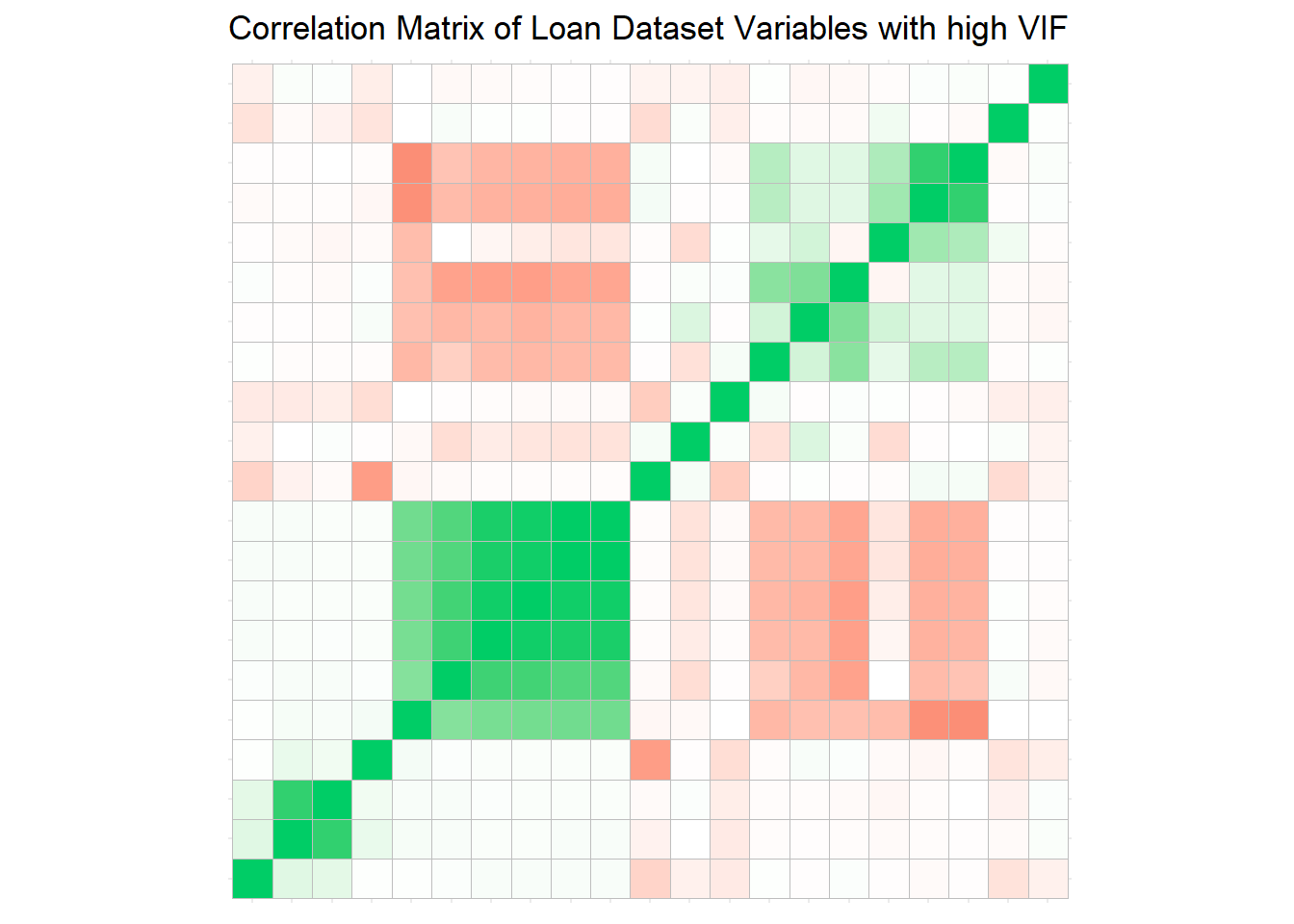
We will now exclude the variables with High VIF maintaining only the variables that are not correlated.
We will use the pairwise correlation indexes to choose the variable to reject, code below will exclude the variable in the pair that have the greater correlation index sum against the other predictors not in the pair beeing evaluated.
At the end we will have only variables that have a correlation index smaller than our selected threshold (0.6).
correl_threshold <- 0.6

reject_variables_vector <- tibble(var_1 = row.names(cor_mtx_high_VIF)) %>%
  bind_cols(as_tibble(cor_mtx_high_VIF)) %>%
  melt(id = c("var_1")) %>%
  filter(var_1 != variable) %>%
  mutate(abs_value = abs(value)) %>%
  filter(abs_value > correl_threshold) %>%
  group_by(var_1) %>%
  mutate(sum_1 = sum(abs_value)) %>%
  ungroup() %>%
  group_by(variable) %>%
  mutate(sum_2 = sum(abs_value)) %>%
  ungroup() %>%
  mutate(reject = ifelse(sum_1 > sum_2, var_1, as.character(variable))) %>%
  distinct(reject)

reject_variables_vector <- reject_variables_vector$reject

clean_dataset <- dplyr::select(loan_dataset_logistic, -reject_variables_vector)

kable(reject_variables_vector)| x |
|---|
| x_district_name_Hl.m._Praha |
| x_no_of_commited_crimes_1996 |
| x_no_of_inhabitants |
| x_no_of_enterpreneurs_per_1000_inhabitants |
| x_region_Prague |
| x_prop_other |
| x_prop_household |
| x_unemploymant_rate_1995 |
| x_transaction_amount |
| x_transaction_count |
| x_no_of_cities |
After the high VIF predictors exclusion we reevaluate the correlation matrix of the original dataset and the cleaned dataset.
Variable names are hidden for readability. Trust us, there is no correlation greater than 0.6 here.
cor_mtx_full <- cor(loan_dataset_logistic)
cor_mtx_clean <- cor(clean_dataset,)

full = ggcorrplot(cor_mtx_full, hc.order = TRUE,
           lab = FALSE,
           lab_size = 3,
           method="square",
           colors = c("tomato2", "white", "springgreen3"),
           title="Correlation Matrix of Full Loan Dataset") +
  theme(axis.text = element_blank(),
        legend.position = 0)

clean = ggcorrplot(cor_mtx_clean, hc.order = TRUE,
           lab = FALSE,
           lab_size = 3,
           method="square",
           colors = c("tomato2", "white", "springgreen3"),
           title="Correlation Matrix of Clean Loan Dataset") +
  theme(axis.text = element_blank(),
        legend.position = 0)

print(ggarrange(full, clean))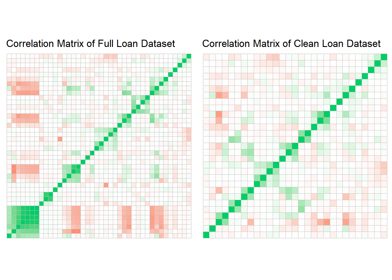
Once again let’s look on the VIF estimates.
vars.quant <- select_if(loan_dataset_logistic, is.numeric)

VIF <- imcdiag(vars.quant, loan_dataset_logistic$y_loan_defaulter)

VIF_Table_After <- tibble(variable = names(VIF$idiags[,1]),
                          VIF = VIF$idiags[,1]) %>%
  arrange(desc(VIF))

ggplot(VIF_Table_After, aes(x = fct_reorder(variable, VIF),
                            y = log(VIF), label = round(VIF, 2))) +
  geom_point(stat='identity', fill="black", size=15)  +
  geom_segment(aes(y = 0,
                   yend = log(VIF),
                   xend = variable),
               color = "black") +
  geom_text(color="white", size=4) +
  geom_hline(aes(yintercept = log(5)), color = 'red', size = 2) +
  scale_y_continuous(labels = NULL, breaks = NULL) +
  coord_flip() +
  theme_economist() +
  theme(legend.position = 'none',
        panel.grid.major = element_blank(),
        panel.grid.minor = element_blank()) +
  labs(x = 'Variable',
       y = NULL,
       title = 'Variance Inflation Factor',
       subtitle="Checking for multicolinearity in X's variables.
       Variables with VIF more than 5 will be droped from the model")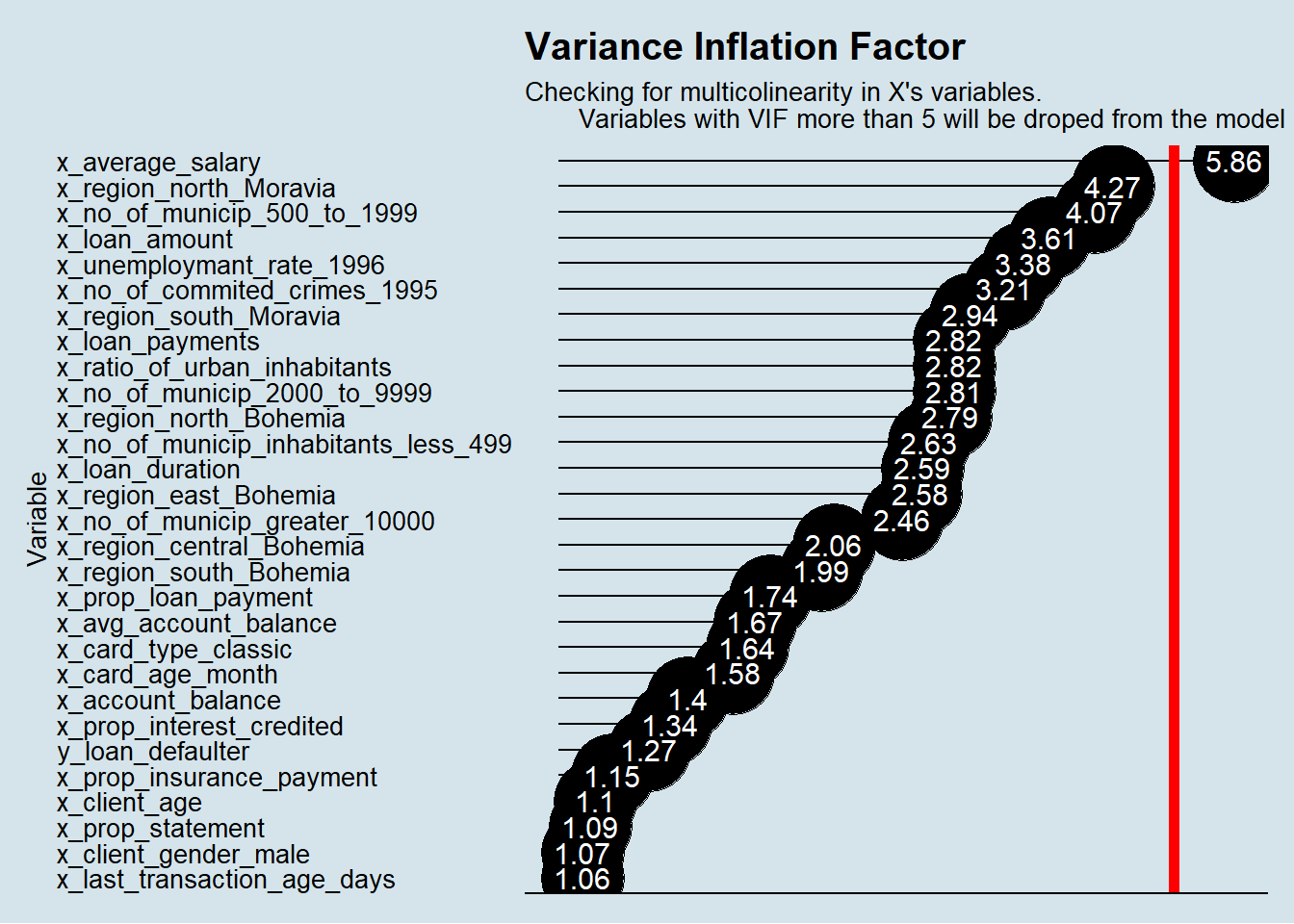
Although x_average_salary have no correlation index greater than our defined threshold (0.6) it still have a VIF greater than 5, and for pure methodological puritanism we decided to exclude this variable as well.
We did try to keep it, but it had no real difference.
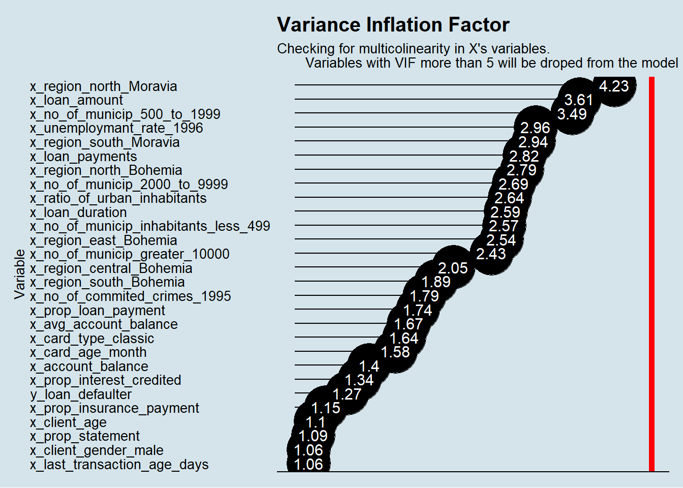
After all this work we end up having 28 variables in the dataset.
| variables |
|---|
| y_loan_defaulter |
| x_account_balance |
| x_avg_account_balance |
| x_card_age_month |
| x_card_type_classic |
| x_client_age |
| x_client_gender_male |
| x_last_transaction_age_days |
| x_loan_amount |
| x_loan_duration |
| x_loan_payments |
| x_no_of_commited_crimes_1995 |
| x_no_of_municip_2000_to_9999 |
| x_no_of_municip_500_to_1999 |
| x_no_of_municip_greater_10000 |
| x_no_of_municip_inhabitants_less_499 |
| x_prop_insurance_payment |
| x_prop_interest_credited |
| x_prop_loan_payment |
| x_prop_statement |
| x_ratio_of_urban_inhabitants |
| x_region_central_Bohemia |
| x_region_east_Bohemia |
| x_region_north_Bohemia |
| x_region_north_Moravia |
| x_region_south_Bohemia |
| x_region_south_Moravia |
| x_unemploymant_rate_1996 |
2.3 Looking for outliers
And what about outliers?
Regression algorithms are known for its sensitivity for outliers. So, before we go for the modeling juice, we will look for those bastards!!!
Looking at the plots we see no significant deviation in the quantitative variables.
x_last_transaction_age_days looks to have a discrepancy, but it is ranging from 0 to 30 days, so it is not real outliers.
# outliers ----------------------------------------------------------------------------
  attach(loan_dataset_logistic)

  par(mfrow=c(2, 3))

  plot(x_last_transaction_age_days, main = "x_last_transaction_age_days", ylab = '')
  plot(x_avg_account_balance, main = "x_avg_account_balance", ylab = '')
  plot(x_account_balance, main = "x_account_balance", ylab = '')
  plot(x_card_age_month, main = "x_card_age_month", ylab = '')
  plot(x_client_age, main = "x_client_age", ylab = '')
  plot(x_loan_amount, main = "x_loan_amount", ylab = '')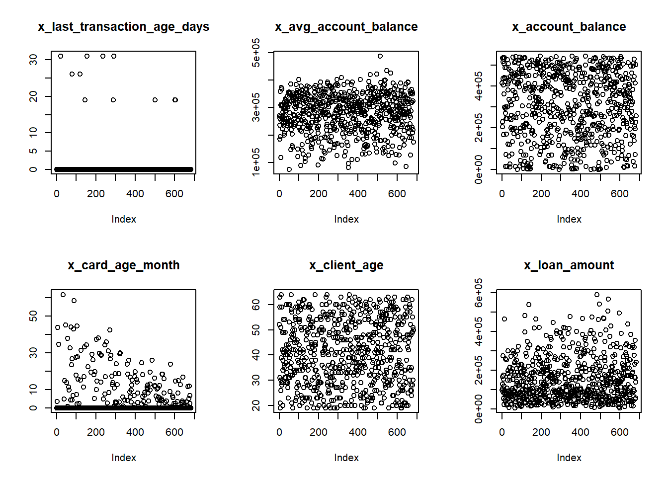
  par(mfrow=c(2, 3))

  plot(x_loan_duration, main = "x_loan_duration", ylab = '')
  plot(x_loan_payments, main = "x_loan_payments", ylab = '')
  plot(x_prop_interest_credited, main = "x_prop_interest_credited", ylab = '')
  plot(x_prop_loan_payment, main = "x_prop_loan_payment", ylab = '')
  plot(x_prop_statement, main = "x_prop_statement", ylab = '')
  plot(x_prop_insurance_payment, main = "x_prop_insurance_payment", ylab = '')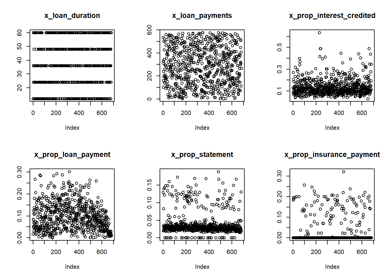
2.4 Sample split into Test and Training Data
The available data in Loan Dataset is split into Train and Testing data on the following proportion:
- Train Dataset (70% 478 obs);
- Test Dataset (30% 204 obs).
SplitDataset <- source_train_test_dataset
data.train_logistic <- SplitDataset$data.train
data.test_logistic <- SplitDataset$data.test

data.train_logistic <- dplyr::select(data.train_logistic, names(loan_dataset_logistic))
data.test_logistic <- dplyr::select(data.test_logistic, names(loan_dataset_logistic))

kable(SplitDataset$event.proportion)| scope | 0 | 1 |
|---|---|---|
| full dataset | 0.8885630 | 0.1114370 |
| train dataset | 0.8933054 | 0.1066946 |
| test dataset | 0.8774510 | 0.1225490 |
Both datasets keep the same proportion for the explained variable around 11%.
This split was saved in disk using the function described in the Data Prep session to be reused in the other models fitted in this exercise.
This will ensure consistency when comparing the models against each other.
2.5 Fit the Logistic Regression model
With the final cleaned dataset, we got from above steps we fit our Logistic Regression model for y_loan_defaulter on all x_variables.
# fit model
logistic.full <- glm(formula = y_loan_defaulter ~ .,
                     data= data.train_logistic,
                     family= binomial(link='logit'))

names(logistic.full$coefficients) <- stringr::str_sub(names(logistic.full$coefficients), 1, 25)
summary(logistic.full)

# save model
saveRDS(logistic.full, './models/logistic_full.rds')
With the full model fitted we will run the stepwise method to automate the selection of predictors using the (Akaike Information Criterion) AIC for short.
This is a broadly used estimator that evaluates the relative quality of statistical methods for a given set of data.
The lower the AIC the better.
logistic.step <- step(logistic.full, direction = "both", test = "F")

names(logistic.step$coefficients) <- stringr::str_sub(names(logistic.step$coefficients), 1, 25)
summary(logistic.step)

# save model
saveRDS(logistic.step, './models/logistic_step.rds')
##
## Call:
## glm(formula = y_loan_defaulter ~ x_card_type_classic + x_loan_amount +
## x_loan_duration + x_no_of_commited_crimes_1995 + x_prop_interest_credited +
## x_prop_statement + x_region_north_Bohemia, family = binomial(link = "logit"),
## data = data.train_logistic)
##
## Deviance Residuals:
## Min 1Q Median 3Q Max
## -1.3847 -0.4555 -0.2810 -0.1517 2.6217
##
## Coefficients:
## Estimate Std. Error z value Pr(>|z|)
## (Intercept) -3.579e+00 6.289e-01 -5.691 1.26e-08 ***
## x_card_type_classic -9.526e-01 6.307e-01 -1.510 0.13094
## x_loan_amount 9.176e-06 1.914e-06 4.794 1.64e-06 ***
## x_loan_duration -3.878e-02 1.467e-02 -2.643 0.00821 **
## x_no_of_commited_crimes_1 -1.650e-02 7.139e-03 -2.311 0.02083 *
## x_prop_interest_credited 1.072e+01 1.895e+00 5.659 1.52e-08 ***
## x_prop_statement 9.416e+00 4.269e+00 2.206 0.02741 *
## x_region_north_Bohemia -1.547e+01 9.701e+02 -0.016 0.98728
## ---
## Signif. codes: 0 '***' 0.001 '**' 0.01 '*' 0.05 '.' 0.1 ' ' 1
##
## (Dispersion parameter for binomial family taken to be 1)
##
## Null deviance: 324.61 on 477 degrees of freedom
## Residual deviance: 249.63 on 470 degrees of freedom
## AIC: 265.63
##
## Number of Fisher Scoring iterations: 173 Interpreting model output
Logistic Regression models are not only good for prediction but also for inference.
Meaning that it can be used not only in predicting the classification into Defaulters and Non-Defaulters but also to understand the relationship between the predictors and the likelihood of delinquency.
In the Logistic Regression the effect of an increase or decrease of a predictor is not linear, but we can see the predictors that have the greater influence and, by its coefficient signal, the association with an increase or decrease on the likelihood of default.
The probability of default is given by below equation:
\[P(Y = 1 | X_{n} = x_{n}) = \frac{1}{1 + e^{-(\beta_{0}+\beta_{1}x_{1}+\beta_{2}x_{2}+...+\beta_{n}x_{n} )}}\]
Where each β is the coefficient estimate for each variable in the final model.
In our model we see that below variables are associated to an increase in the likelihood of default:
- x_loan_amount
- x_prop_interest_credited
- x_prop_statement
On the other hand, below variables are associated to a decrease in the likelihood of default:
- x_card_type_classic
- x_loan_duration
- x_no_of_commited_crimes_1995
- x_loan_amount
- x_region_north_Bohemia
4 Evaluating the model performance
We started this step by making predictions using our model on the X’s variables in our Train and Test datasets.
## making predictions for each model and consolidating in a single data frame

prob.full   = list()
prob.train  = list()
prob.test   = list()

prob.full$logistic.actual     <- loan_dataset_logistic$y_loan_defaulter
prob.full$logistic.predicted  <- predict(logistic.step, type = "response",
                                         newdata = loan_dataset_logistic)

prob.train$logistic.actual    <- data.train_logistic$y_loan_defaulter
prob.train$logistic.predicted <- predict(logistic.step, type = "response",
                                         newdata = data.train_logistic)

prob.test$logistic.actual     <- data.test_logistic$y_loan_defaulter
prob.test$logistic.predicted  <- predict(logistic.step, type = "response",
                                         newdata = data.test_logistic)

prob.full   <- prob.full  %>% as_tibble()
prob.train  <- prob.train %>% as_tibble()
prob.test   <- prob.test  %>% as_tibble()
4.1 Getting Performance Measures
To calculate the performance measures, derived from the confusion matrix, we need to find the score cut off that best split our test dataset into Defaulters and Non-Defaulters.
In this exercise we decide to not prioritize the accuracy on predicting Defaulters and Non-Defaulters, therefore we are looking for the score cut off that best predict each class equally.
We will use the custom functions described in Auxiliary metrics functions topic in the Data Preparation session of this site.
With the returned object from this function we can plot the comparison between TPR (True Positive Rate) and TNR (True Negative Rate) to find the best cut off.
## getting measures -----------------------------------------------------------------

metricsByCutoff.test_log    <- modelMetrics(prob.test$logistic.actual,
                                            prob.test$logistic.predicted,
                                            plot_title = 'Logistic Regression')
metricsByCutoff.test_log$Plot
With the optimized cut off we calculate the full set of model metrics using the function HMeasure from hmeasure library.
# logistic regression
measures.logistic.train <- HMeasure(prob.train$logistic.actual,
                                    prob.train$logistic.predicted,
                                    threshold = metricsByCutoff.test_log$BestCut['Cut'])
measures.logistic.test <- HMeasure(prob.test$logistic.actual,
                                   prob.test$logistic.predicted,
                                   threshold = metricsByCutoff.test_log$BestCut['Cut'])

# join measures in a single data frame
measures <- t(bind_rows(measures.logistic.train$metrics,
                        measures.logistic.test$metrics)
              ) %>% as_tibble(., rownames = NA)

colnames(measures) <- c('logistic - train', 'logistic - test')

measures$metric = rownames(measures)

measures <- dplyr::select(measures, metric, everything())
Below are the metrics on the train and test dataset:
| metric | logistic - train | logistic - test |
|---|---|---|
| H | 0.3612900 | 0.3070793 |
| Gini | 0.6641411 | 0.5195531 |
| AUC | 0.8320705 | 0.7597765 |
| AUCH | 0.8475456 | 0.7915084 |
| KS | 0.5492033 | 0.4370950 |
| MER | 0.0920502 | 0.1078431 |
| MWL | 0.0859316 | 0.1210592 |
| Spec.Sens95 | 0.5339578 | 0.3072626 |
| Sens.Spec95 | 0.3725490 | 0.3200000 |
| ER | 0.3347280 | 0.3333333 |
| Sens | 0.8431373 | 0.6400000 |
| Spec | 0.6440281 | 0.6703911 |
| Precision | 0.2205128 | 0.2133333 |
| Recall | 0.8431373 | 0.6400000 |
| TPR | 0.8431373 | 0.6400000 |
| FPR | 0.3559719 | 0.3296089 |
| F | 0.3495935 | 0.3200000 |
| Youden | 0.4871654 | 0.3103911 |
| TP | 43.0000000 | 16.0000000 |
| FP | 152.0000000 | 59.0000000 |
| TN | 275.0000000 | 120.0000000 |
| FN | 8.0000000 | 9.0000000 |
4.2 Evaluating classification performance
In general the Logistic Regression model is not delivering good accuracy, we will compare how it performed against other classes of models in the Final Report session
Below the confusion matrix and general performance of the model using our custom function accuracy described in Auxiliary metrics functions topic in the Data Preparation session of this site.
# accuracy metrics ---------------------------------------------------------------
# logistic regression
accuracy(score = prob.test$logistic.predicted,
         actual = prob.test$logistic.actual,
         threshold = metricsByCutoff.test_log[["BestCut"]][["Cut"]])
##
##
## pred.1 pred.0
## --------- ------- -------
## actual.1 16 9
## actual.0 59 120
## [1] "--------------------------------------------------------------"
## [1] "Model General Accuracy of: 66.67%"
## [1] "True Positive Rate of : 64%"We finally look at the score distribution charts to check how well the model is able to discriminate Defaulters and Non-Defaulters.
p1 <- Score_Histograms(prob.test,
                 prob.test$logistic.predicted,
                 prob.test$logistic.actual,
                 'Density Plot') + theme(axis.title.y = element_blank())

p2 <- Score_Boxplot(prob.test,
              prob.test$logistic.predicted,
              prob.test$logistic.actual,
              'Score Boxplot')

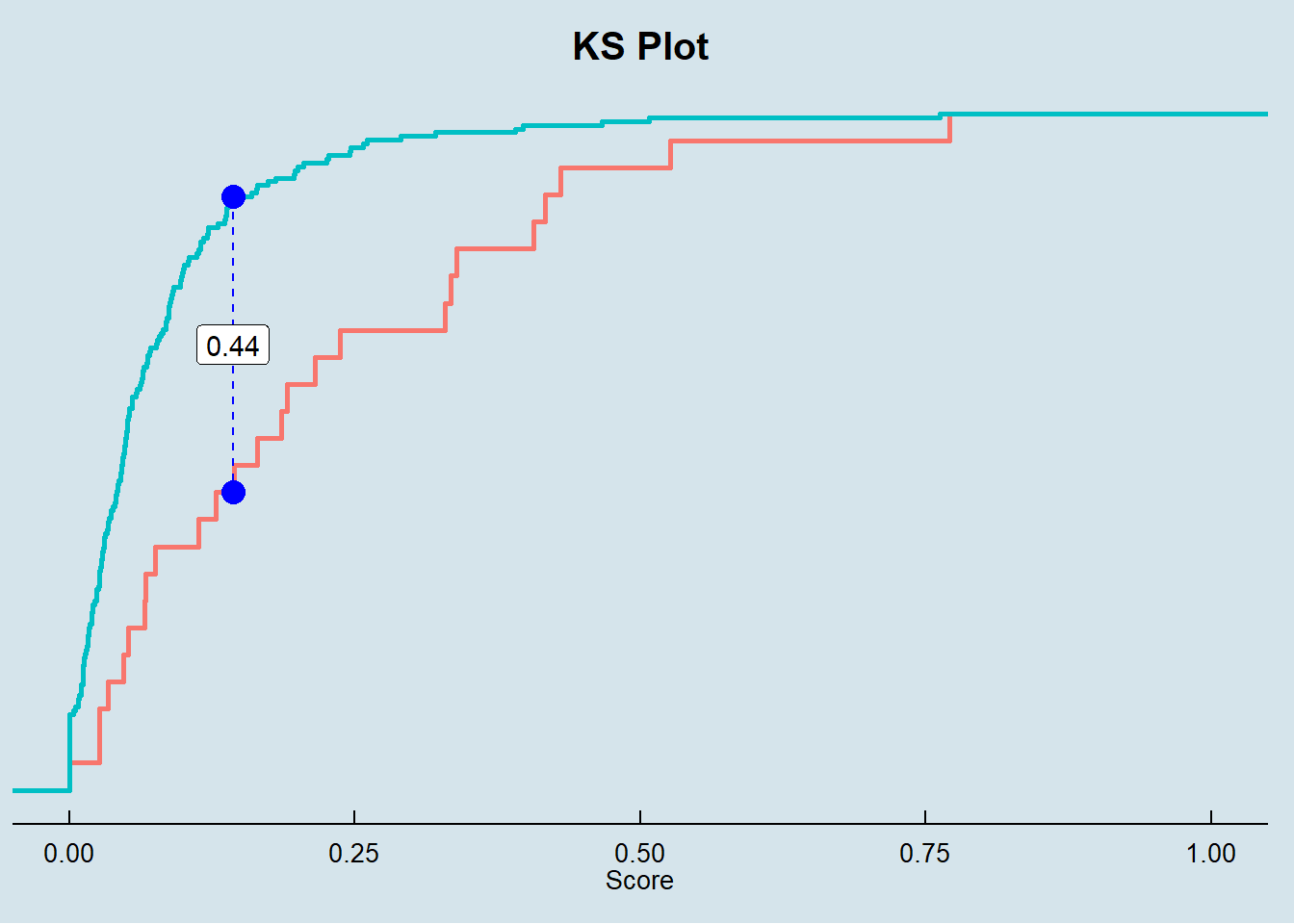
p3 <- KS_Plot(prob.test$logistic.predicted[prob.test$logistic.actual == 0],
        prob.test$logistic.predicted[prob.test$logistic.actual == 1],
        'KS Plot') + theme(axis.title.y = element_blank(),
                           axis.text.y = element_blank())
ggarrange(p1, p2, nrow = 2)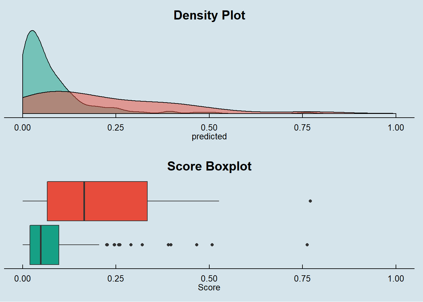
By the score density we see that our Logistic Regression model is very broad on the scores it assigns to the observations, especially for the real Defaulters not providing a good separation between each class.
The box plot also does not show a clear discrimination between Defaulters and Non-Defaulters.
Finally, the KS metric is far from what is expected for a reasonable classification model.
In the Final Report session, we will look more closely on the AUC and Gini metrics by plotting the ROC curve and comparing against other models.