The exploration’s report

1 Gender Exploration

At first glance, gender equality is well balanced in the bank, even when observed over the decades. Even more impressive, gender equality is everywhere in the country.

# gender distribution of clients in the bank
gender_plot <- ggplot(data = client) +
  aes(x = gender, fill = gender) +
  geom_bar() +
  labs(subtitle = "A well balanced bank",
       x = "Gender",
       y = "Total clients") +
  theme_economist()

clientGenderOverDecades <- client %>% 
  group_by(decade = as.integer(substr(client$birth_number, 1,1)) * 10, 
           gender = client$gender) %>% 
  count()

# gender distribution of clients in the bank over the decades
gender_dist_plot <- ggplot(data = clientGenderOverDecades) +
  aes(x = decade, fill = gender, weight = n) +
  scale_x_continuous(breaks = c(0, 10, 20, 30, 40, 50, 60, 70, 80)) +
  geom_bar() +
  geom_line(aes(y = n, color = gender)) +
  labs(subtitle = "Equality at its finest",
       x = "Decades",
       y = "Total clients") +
  theme_economist() +
  facet_wrap(vars(gender))

gender_plots <- ggarrange(gender_plot, gender_dist_plot)

gender_plots <- annotate_figure(gender_plots, 
                                 top = text_grob("Gender distribution of clients over the decades", 
                                                 color = "black", face = "bold", 
                                                 size = 14))
gender_plots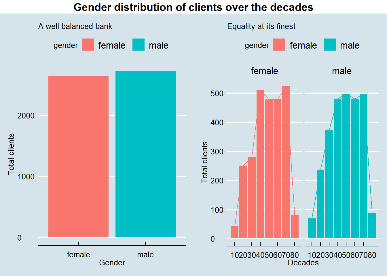

# alluvial diagram representation of gender, age group and region
clientGenderAgeGroupByRegion <- client %>% 
  mutate(age_group = ifelse(age < 21, "young", 
                     ifelse(age >= 21 & age <= 60, "adult", "senior"))) %>% 
  inner_join(district, by = "district_id") %>% 
  group_by(age_group, gender, region) %>% 
  count()
  
ggplot(data = clientGenderAgeGroupByRegion, 
       aes(axis1 = region, axis2 = age_group, y = n)) +
  scale_x_discrete(limits = c("region", "age group"), expand = c(.1, .1)) +
  xlab("Demographic") +
  geom_alluvium(aes(fill = gender), knot.pos = 0) +
  geom_stratum() + 
  geom_text(stat = "stratum", label.strata = TRUE) +
  theme_economist() +
  ggtitle("Region and age group by gender", "Equality is everywhere")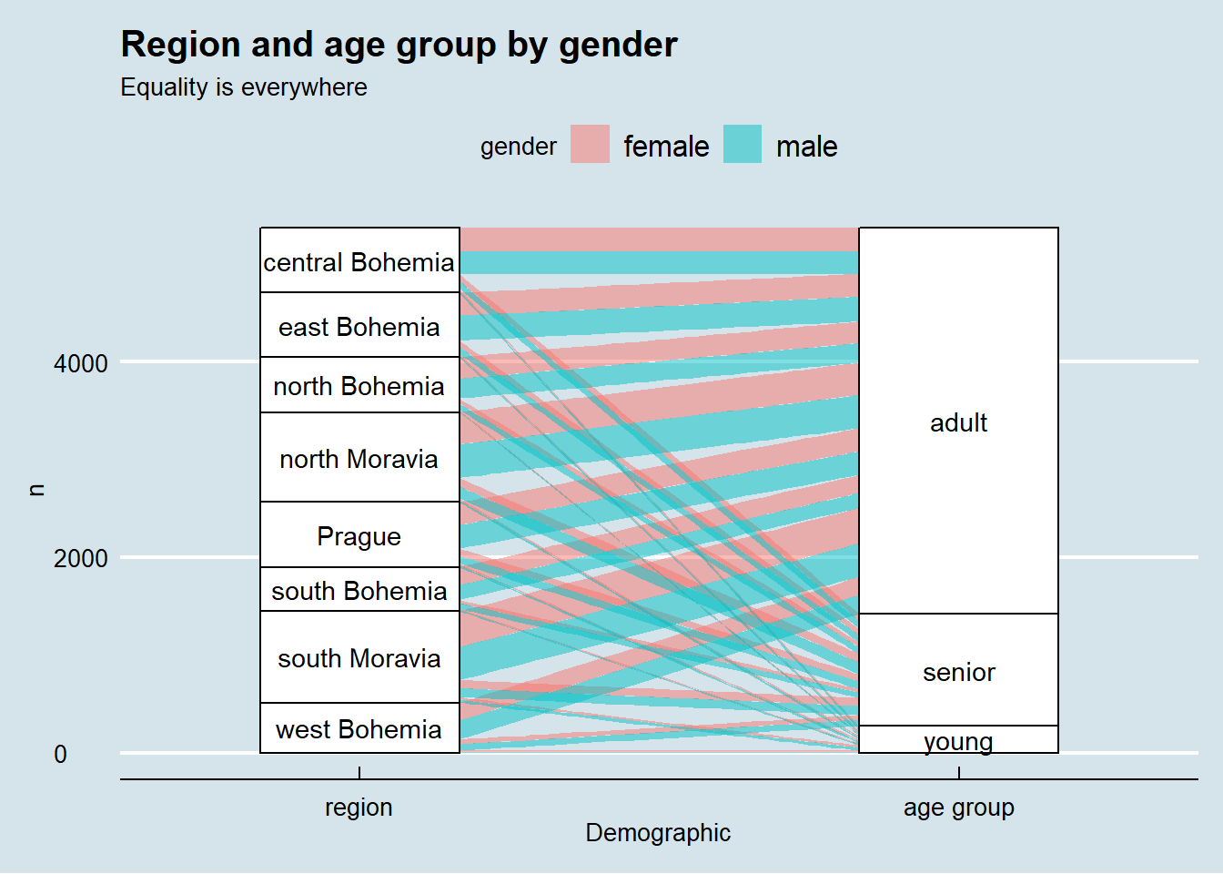 

2 Loan Exploration

Here we investigate if there is any association between the region and the likelihood of default in the 682 loan observations in the dataset.

left_join(loan, disposition, by = 'account_id') %>% 
  left_join(client, by = 'client_id') %>% 
  left_join(district, by = 'district_id') %>% 
  group_by(region, contract_status, defaulter) %>% 
  summarise(count = n(),
            amount = sum(amount)) %>% 
  group_by(region, contract_status) %>% 
  mutate(count_contract_status = sum(count),
         amount_contract_status = sum(amount)) %>% 
  group_by(region) %>% 
  mutate(count_region = sum(count),
         amount_region = sum(amount)) %>% 
  ggplot(aes(x = defaulter, y = contract_status, fill = count / count_region)) +
  geom_bin2d(stat = 'identity') +
  geom_text(aes(label = paste(round(count / count_region * 100, 2), '%')), 
            color = 'white') +
  facet_wrap(~region) +
  theme_economist() +
  theme(legend.position = 'none', panel.grid.major = element_blank(), 
        panel.grid.minor = element_blank()) +
  labs(x = 'Defaulter', 
       y = 'Contract Status', 
       title = 'Loan Contract Status by Region Heatmap')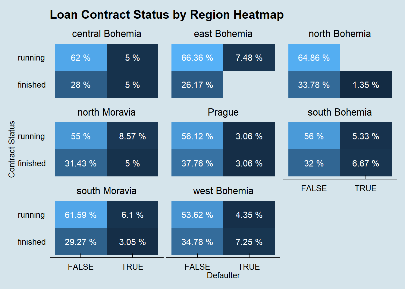

We perform the same investigation on the association between the client gender and the likelihood of default in the 682 loan observations in the dataset.

left_join(loan, disposition, by = 'account_id') %>%
  left_join(client, by = 'client_id') %>% 
  left_join(district, by = 'district_id') %>% 
  group_by(gender, contract_status, defaulter) %>% 
  summarise(count = n(),
            amount = sum(amount)) %>% 
  group_by(gender, contract_status) %>% 
  mutate(count_contract_status = sum(count),
         amount_contract_status = sum(amount)) %>% 
  group_by(gender) %>% 
  mutate(count_gender = sum(count),
         amount_gender = sum(amount)) %>% 
  ggplot(aes(x = defaulter, y = contract_status, 
             fill = count / count_gender)) +
    geom_bin2d(stat = 'identity') +
    geom_text(aes(label = paste(round(count / count_gender * 100, 2), '%')), 
              color = 'white') +
    facet_wrap(~gender) +
    theme_economist() +
    theme(legend.position = 'none', panel.grid.major = element_blank(), 
          panel.grid.minor = element_blank()) +
    labs(x = 'Defaulter',
         y = 'Contract Status',
         title = 'Loan Contract Status by Gender Heatmap')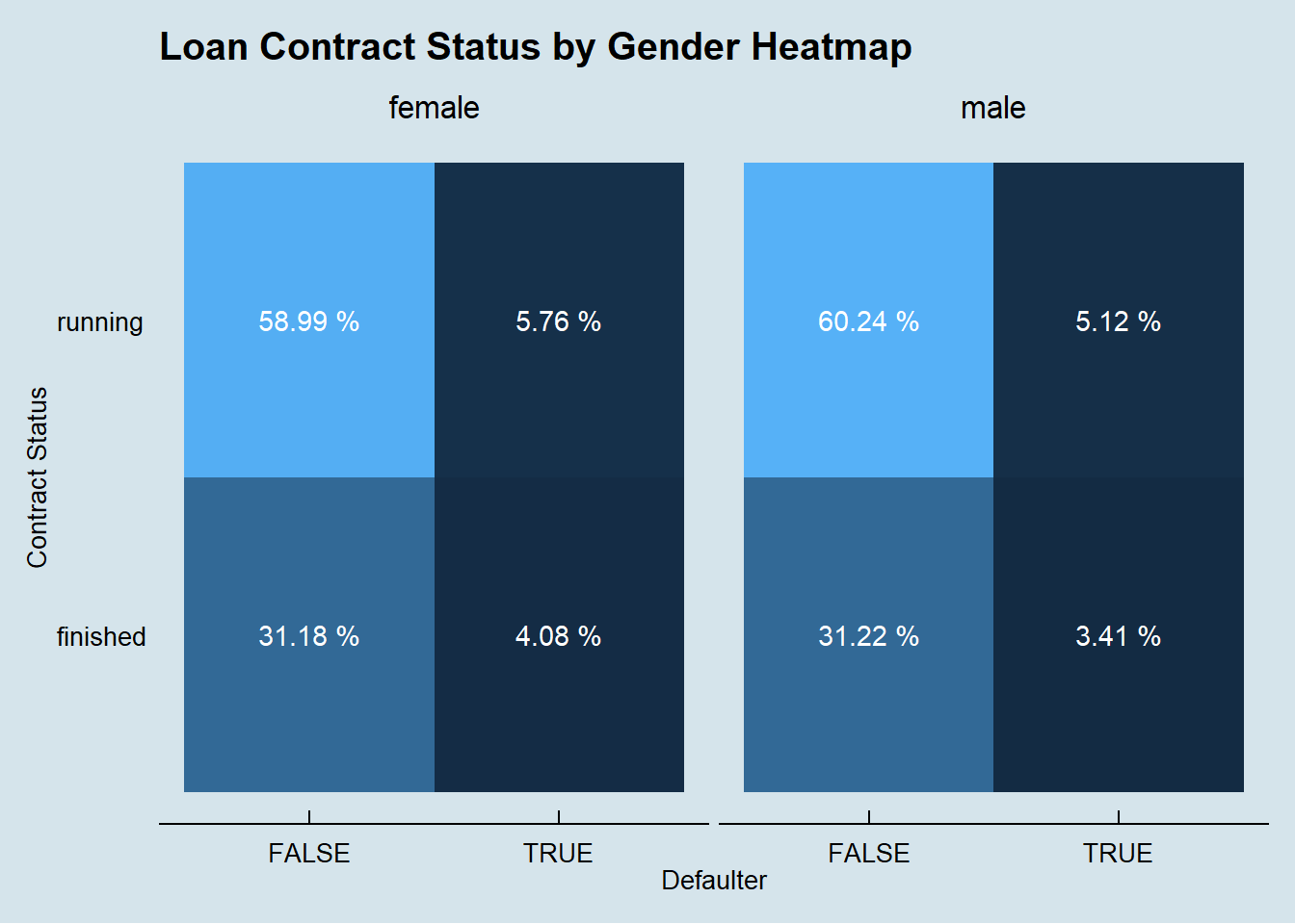

We finnaly do the same investigation on the association between the client age and the likelihood of default in the 682 loan observations in the dataset.

left_join(loan, disposition, by = 'account_id') %>%
  left_join(client, by = 'client_id') %>% 
  left_join(district, by = 'district_id') %>% 
  group_by(age_bin, contract_status, defaulter) %>% 
  summarise(count = n(),
            amount = sum(amount)) %>% 
  group_by(age_bin, contract_status) %>% 
  mutate(count_contract_status = sum(count),
         amount_contract_status = sum(amount)) %>% 
  group_by(age_bin) %>% 
  mutate(count_age_bin = sum(count),
         amount_age_bin = sum(amount)) %>% 
  ggplot(aes(x = defaulter, 
             y = contract_status, fill = count / count_age_bin)) +
    geom_bin2d(stat = 'identity') +
    geom_text(aes(label = paste(round(count / count_age_bin * 100, 2), '%')), 
              color = 'white') +
    facet_wrap(~age_bin) +
    theme_economist() +
    theme(legend.position = 'none', panel.grid.major = element_blank(), 
          panel.grid.minor = element_blank()) +
    labs(x = 'Defaulter',
         y = 'Contract Status',
         title = 'Loan Contract Status by Age Group Heatmap')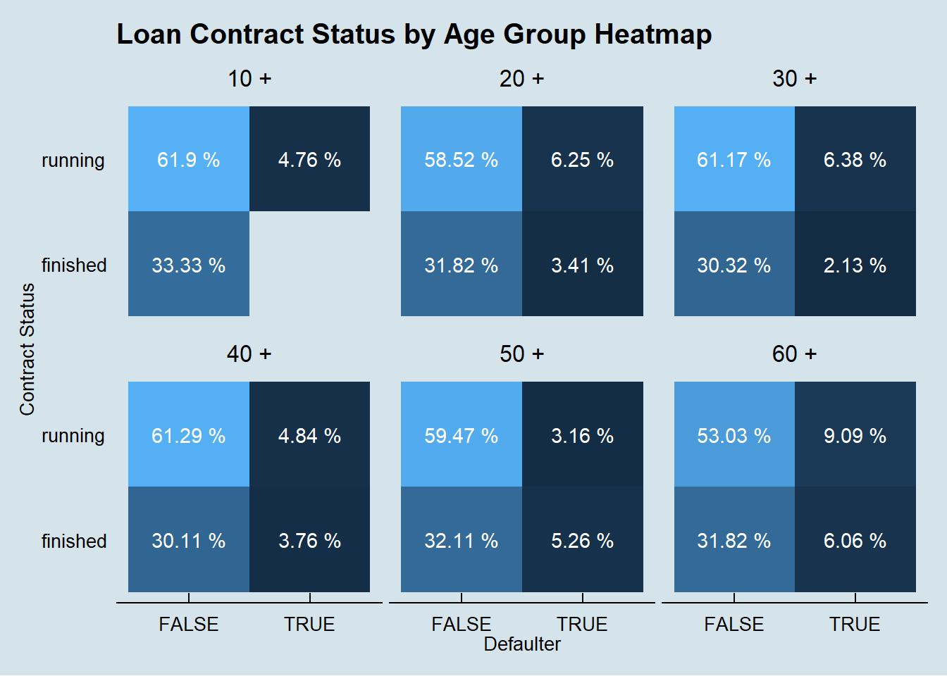

It seems that none of these features, alone, are determinant on the odds of a client default.

3 Account Balance Exploration

As we do not have the individual income of each client, we tried to perform a proxy of the client’s wealth by calculating the average account balance of each account and investigating the distribution by region and age.

left_join(account_balance, disposition, by = 'account_id') %>%
  left_join(client, by = 'client_id') %>% 
  left_join(district, by = 'district_id') %>% 
  filter(type == 'Owner') %>% 
  ggplot(aes(avg_balance / 1000)) +
    geom_density(alpha = 0.5, aes(fill = gender)) +
    scale_x_continuous(labels = scales::comma) +
    labs(title = 'Average Account Balance Distribution by Gender and Region',
         subtitle = 'k (Kč) - Koruna (CZK)') +
    theme_economist() +
    facet_wrap(~region)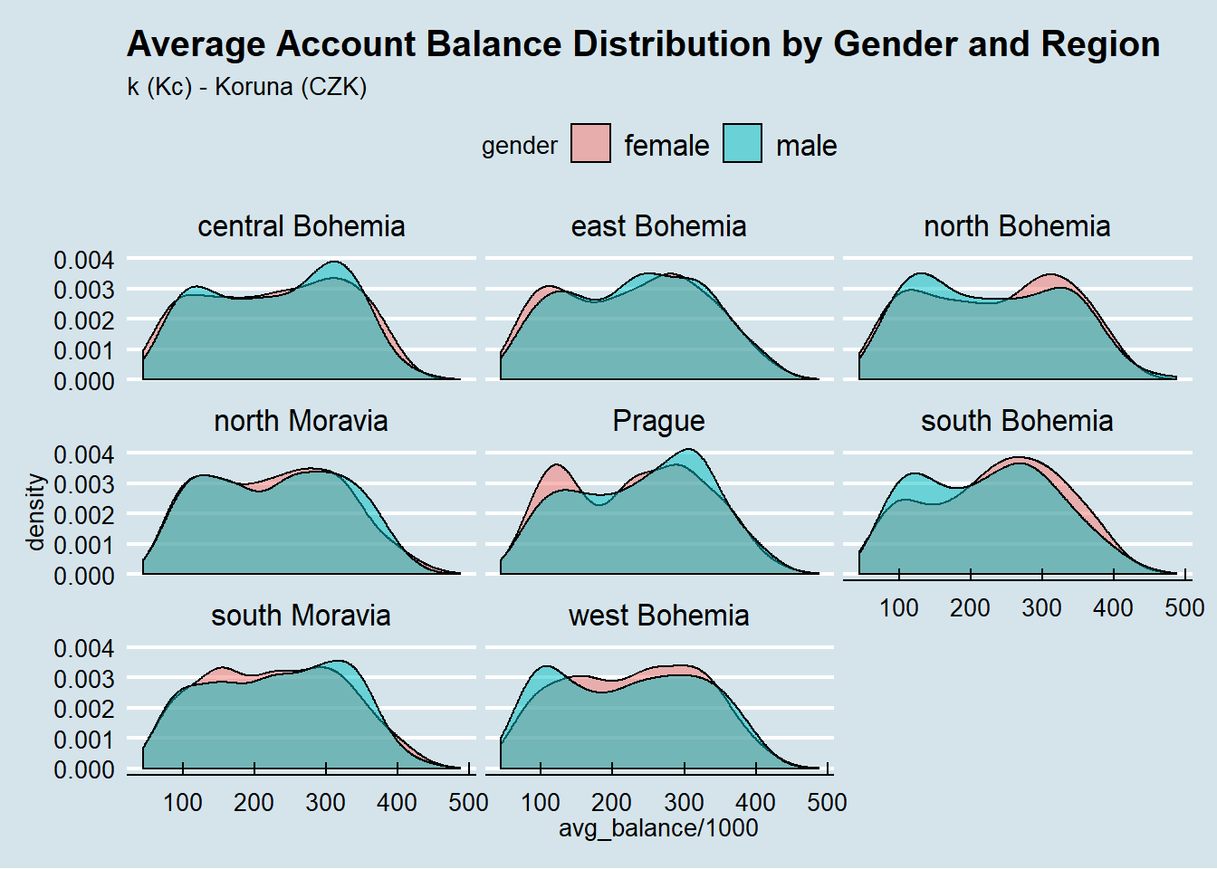

One interest pattern shows up, males in prague region tend to have a bigger average account balance them females, and the oposite trend in South, North and West Bohemia.

4 District exploration

Regarding the Czech regions, we can notice in the exploration below which regions are more likely to have defaulters based on the finished loans operations so far.

loan_amount_by_region <- dplyr::select(loan, account_id, amount, defaulter, contract_status) %>% 
  filter(defaulter == TRUE) %>% 
  inner_join(account) %>% 
  inner_join(district) %>% 
  group_by(region) %>% 
  summarise(transaction_count = n(),
            amount = sum(amount)) %>% 
  inner_join(czech_regions_coords)

jsonMapFile <- "./map/czech-republic-regions.json"
czech_regions <- as.json(geojson_read(jsonMapFile))

leaflet(loan_amount_by_region) %>% 
  addTiles() %>% 
  setView(lng = 15.3, lat = 49.8, zoom = 7) %>%
  addGeoJSON(czech_regions, fillColor = "red", stroke = "#555555") %>% 
  addCircles(lng = ~long,   
             lat = ~lat,    
             weight = 2,    
             radius = ~sqrt(amount) * 30,   
             popup = ~region)