Aplicando os modelos SAR e GWR
Junho de 2020
1 Carregamento do shapefile, preparação e análises iniciais
O primeiro passo é o carregamento do shapefile, previamente preparado nas etapas anteriores, para iniciarmos uma análise iniciai quanto as variáveis.
dataProcessedDirectory <- "./data/processed/"
shapefile_to_read <- paste(dataProcessedDirectory,
                           "gas_prices_hist",
                           sep = "")
target <- readOGR(shapefile_to_read, encoding="UTF-8")
## OGR data source with driver: ESRI Shapefile
## Source: "D:\rodri\My GIT Projects\Spatial-Statistics-Applications\data\processed\gas_prices_hist", layer: "gas_prices_hist"
## with 458 features
## It has 42 fieldsdatatable(data = target@data[,c("CodIBGE", "Regiao", "Estado", "Cidade", "NmPostPesq", "PcMedRev")],
style = 'bootstrap',
options = list(pageLength = 10,autoWidth = TRUE))1.1 Variáveis presentes no dataset
Abaixo, vemos uma lista das variáveis presente no dataset do shapefile analisado.
1.2 Calculando os centróides e a matrix de vizinhança
Em seguida, obtém-se os centroides do shapefile para gerar a matriz de vizinhança dos polígonos espaciais e polígonos adjacentes através da biblioteca spdep usando a primeira ordem. A biblioteca bamlss será usada para gerar a matriz de vizinhança, baseada em um k = 3 . O plot mostra o resultado desta configuração inicial.
xy <- coordinates(target)

ap <- poly2nb(target, queen = T, row.names = target$Index)
lw <- nb2listw(ap, style = "W", zero.policy = TRUE)
nm <- neighbormatrix(target, type = "boundary", k = 3)

plotneighbors(target, type = "delaunay")
##
## PLEASE NOTE: The components "delsgs" and "summary" of the
## object returned by deldir() are now DATA FRAMES rather than
## matrices (as they were prior to release 0.0-18).
## See help("deldir").
##
## PLEASE NOTE: The process that deldir() uses for determining
## duplicated points has changed from that used in version
## 0.0-9 of this package (and previously). See help("deldir").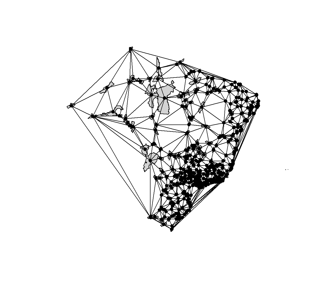
2 Aplicando os modelos
Nas etapas a seguir, serão aplicados vários modelos a fim de entendermos se existe relacionamento espacial entre as variáveis do shapefile.
2.1 Implementando o modelo de regressão linear multivariado stepwise
Iniciamos por avaliar a relação do preço médio de revenda com a distância média para as 10 refinarias mais próximas..
# initial exploration in PcMedRev x DistMean
pcmedrev_by_DistMean_plot <- ggplot(data = target@data,
                                    aes(x = target$DistMean,
                                        y = target$PcMedRev,
                                        color = target$DistMean)) +
  geom_point() +
  theme(legend.position = "none") +
  xlab("DistMean") +
  ylab("PcMedRev")

ggMarginal(pcmedrev_by_DistMean_plot, type = "histogram")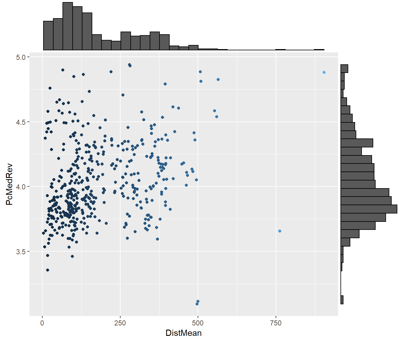
Na sequencia implementamos um modelo com todas as variáveis que julgamos serem relevantes para o estudo.
# runing the lm multivaluated model
target.lm.multivaluated.model <- lm(PcMedRev ~
                                      DistMean +
                                      DistDev +
                                      DistMin +
                                      RefinMean +
                                      RefinDev +
                                      RefinMin +
                                      RefinMax +
                                      ChgPIB +
                                      ChgPIBCap +
                                      PIB_2016 +
                                      PIB_2017 +
                                      PIBCap2016 +
                                      PIBCap2017 +
                                      PopEst,
                                    data = target)

summary(target.lm.multivaluated.model)
##
## Call:
## lm(formula = PcMedRev ~ DistMean + DistDev + DistMin + RefinMean +
## RefinDev + RefinMin + RefinMax + ChgPIB + ChgPIBCap + PIB_2016 +
## PIB_2017 + PIBCap2016 + PIBCap2017 + PopEst, data = target)
##
## Residuals:
## Min 1Q Median 3Q Max
## -1.19222 -0.15259 -0.01514 0.15023 0.84979
##
## Coefficients:
## Estimate Std. Error t value Pr(>|t|)
## (Intercept) 3.907e+00 1.193e-01 32.765 < 2e-16 ***
## DistMean 8.561e-04 2.711e-04 3.158 0.001698 **
## DistDev -2.576e-03 4.962e-04 -5.191 3.2e-07 ***
## DistMin -8.411e-04 2.990e-04 -2.813 0.005128 **
## RefinMean -2.311e-04 7.397e-05 -3.124 0.001900 **
## RefinDev -1.850e-03 1.634e-04 -11.320 < 2e-16 ***
## RefinMin -2.983e-04 7.666e-05 -3.891 0.000115 ***
## RefinMax 7.790e-04 8.202e-05 9.497 < 2e-16 ***
## ChgPIB -6.071e+00 2.094e+00 -2.899 0.003936 **
## ChgPIBCap 6.192e+00 2.113e+00 2.931 0.003557 **
## PIB_2016 -1.242e-08 2.580e-08 -0.481 0.630527
## PIB_2017 1.406e-08 2.516e-08 0.559 0.576432
## PIBCap2016 7.994e-07 7.096e-06 0.113 0.910352
## PIBCap2017 -1.823e-06 7.111e-06 -0.256 0.797802
## PopEst -1.304e-07 6.947e-08 -1.877 0.061212 .
## ---
## Signif. codes: 0 '***' 0.001 '**' 0.01 '*' 0.05 '.' 0.1 ' ' 1
##
## Residual standard error: 0.2496 on 443 degrees of freedom
## Multiple R-squared: 0.3387, Adjusted R-squared: 0.3178
## F-statistic: 16.21 on 14 and 443 DF, p-value: < 2.2e-16Chamamos de stepwise uma modificação da seleção forward em que cada passo todas as variáveis do modelo são previamente verificadas pelas suas estatísticas \(F\) parciais. Uma variável adicionada no modelo no passo anterior pode ser redundante para o modelo por causa do seu relacionamento com as outras variáveis e se sua estatística \(F\) parcial for menor que \(F_{out}\), ela é removida do modelo.
Procedimento:
- Iniciamos com uma variável: aquela que tiver maior correlação com a variável resposta;
- A cada passo do forward, depois de incluir uma variável, aplica-se o backward para ver se será descartada alguma variável;
- Continuamos o processo até não incluir ou excluir nenhuma variável.
Assim, a regressão Stepwise requer dois valores de corte: \(F_{in}\) e \(F_{out}\). Alguns autores preferem escolher \(F_{in}=F_{out}\) mas isso não é necessário. Se \(F_{in} < F_{out}\): mais difícil remover que adicionar; se \(F_{in} > F_{out}\): mais difícil adicionar que remover.
# performing the stepwise selection
target.lm.multivaluated.stepwise <- step(target.lm.multivaluated.model,
                                         direction = c("both", "backward", "forward"),
                                         k = 2)
## Start: AIC=-1256.56
## PcMedRev ~ DistMean + DistDev + DistMin + RefinMean + RefinDev +
## RefinMin + RefinMax + ChgPIB + ChgPIBCap + PIB_2016 + PIB_2017 +
## PIBCap2016 + PIBCap2017 + PopEst
##
## Df Sum of Sq RSS AIC
## - PIBCap2016 1 0.0008 27.600 -1258.5
## - PIBCap2017 1 0.0041 27.604 -1258.5
## - PIB_2016 1 0.0144 27.614 -1258.3
## - PIB_2017 1 0.0195 27.619 -1258.2
## <none> 27.599 -1256.6
## - PopEst 1 0.2194 27.819 -1254.9
## - DistMin 1 0.4929 28.092 -1250.5
## - ChgPIB 1 0.5234 28.123 -1250.0
## - ChgPIBCap 1 0.5351 28.135 -1249.8
## - RefinMean 1 0.6081 28.208 -1248.6
## - DistMean 1 0.6212 28.221 -1248.4
## - RefinMin 1 0.9434 28.543 -1243.2
## - DistDev 1 1.6785 29.278 -1231.5
## - RefinMax 1 5.6197 33.219 -1173.7
## - RefinDev 1 7.9830 35.582 -1142.2
##
## Step: AIC=-1258.54
## PcMedRev ~ DistMean + DistDev + DistMin + RefinMean + RefinDev +
## RefinMin + RefinMax + ChgPIB + ChgPIBCap + PIB_2016 + PIB_2017 +
## PIBCap2017 + PopEst
##
## Df Sum of Sq RSS AIC
## - PIB_2016 1 0.0148 27.615 -1260.3
## - PIB_2017 1 0.0206 27.621 -1260.2
## <none> 27.600 -1258.5
## - PIBCap2017 1 0.1802 27.780 -1257.6
## - PopEst 1 0.2197 27.820 -1256.9
## + PIBCap2016 1 0.0008 27.599 -1256.6
## - DistMin 1 0.4924 28.093 -1252.4
## - ChgPIB 1 0.5230 28.123 -1251.9
## - ChgPIBCap 1 0.5372 28.137 -1251.7
## - RefinMean 1 0.6074 28.208 -1250.6
## - DistMean 1 0.6214 28.222 -1250.3
## - RefinMin 1 0.9498 28.550 -1245.0
## - DistDev 1 1.6789 29.279 -1233.5
## - RefinMax 1 5.6191 33.219 -1175.7
## - RefinDev 1 8.0175 35.618 -1143.7
##
## Step: AIC=-1260.3
## PcMedRev ~ DistMean + DistDev + DistMin + RefinMean + RefinDev +
## RefinMin + RefinMax + ChgPIB + ChgPIBCap + PIB_2017 + PIBCap2017 +
## PopEst
##
## Df Sum of Sq RSS AIC
## <none> 27.615 -1260.3
## - PIB_2017 1 0.1448 27.760 -1259.9
## - PIBCap2017 1 0.1869 27.802 -1259.2
## - PopEst 1 0.2222 27.837 -1258.6
## + PIB_2016 1 0.0148 27.600 -1258.5
## + PIBCap2016 1 0.0011 27.614 -1258.3
## - DistMin 1 0.4966 28.112 -1254.1
## - ChgPIB 1 0.5103 28.125 -1253.9
## - ChgPIBCap 1 0.5225 28.137 -1253.7
## - RefinMean 1 0.5991 28.214 -1252.5
## - DistMean 1 0.6158 28.231 -1252.2
## - RefinMin 1 0.9518 28.567 -1246.8
## - DistDev 1 1.6834 29.298 -1235.2
## - RefinMax 1 5.6141 33.229 -1177.5
## - RefinDev 1 8.0235 35.639 -1145.5##
## Call:
## lm(formula = PcMedRev ~ DistMean + DistDev + DistMin + RefinMean +
## RefinDev + RefinMin + RefinMax + ChgPIB + ChgPIBCap + PIB_2017 +
## PIBCap2017 + PopEst, data = target)
##
## Residuals:
## Min 1Q Median 3Q Max
## -1.19434 -0.15170 -0.01271 0.14350 0.85010
##
## Coefficients:
## Estimate Std. Error t value Pr(>|t|)
## (Intercept) 3.906e+00 1.187e-01 32.896 < 2e-16 ***
## DistMean 8.520e-04 2.704e-04 3.150 0.001741 **
## DistDev -2.579e-03 4.952e-04 -5.208 2.92e-07 ***
## DistMin -8.439e-04 2.983e-04 -2.829 0.004882 **
## RefinMean -2.288e-04 7.363e-05 -3.107 0.002010 **
## RefinDev -1.852e-03 1.628e-04 -11.371 < 2e-16 ***
## RefinMin -2.991e-04 7.638e-05 -3.916 0.000104 ***
## RefinMax 7.786e-04 8.185e-05 9.511 < 2e-16 ***
## ChgPIB -5.835e+00 2.035e+00 -2.868 0.004333 **
## ChgPIBCap 5.987e+00 2.063e+00 2.902 0.003897 **
## PIB_2017 1.973e-09 1.292e-09 1.527 0.127384
## PIBCap2017 -1.042e-06 6.003e-07 -1.735 0.083393 .
## PopEst -1.311e-07 6.931e-08 -1.892 0.059126 .
## ---
## Signif. codes: 0 '***' 0.001 '**' 0.01 '*' 0.05 '.' 0.1 ' ' 1
##
## Residual standard error: 0.2491 on 445 degrees of freedom
## Multiple R-squared: 0.3383, Adjusted R-squared: 0.3205
## F-statistic: 18.96 on 12 and 445 DF, p-value: < 2.2e-16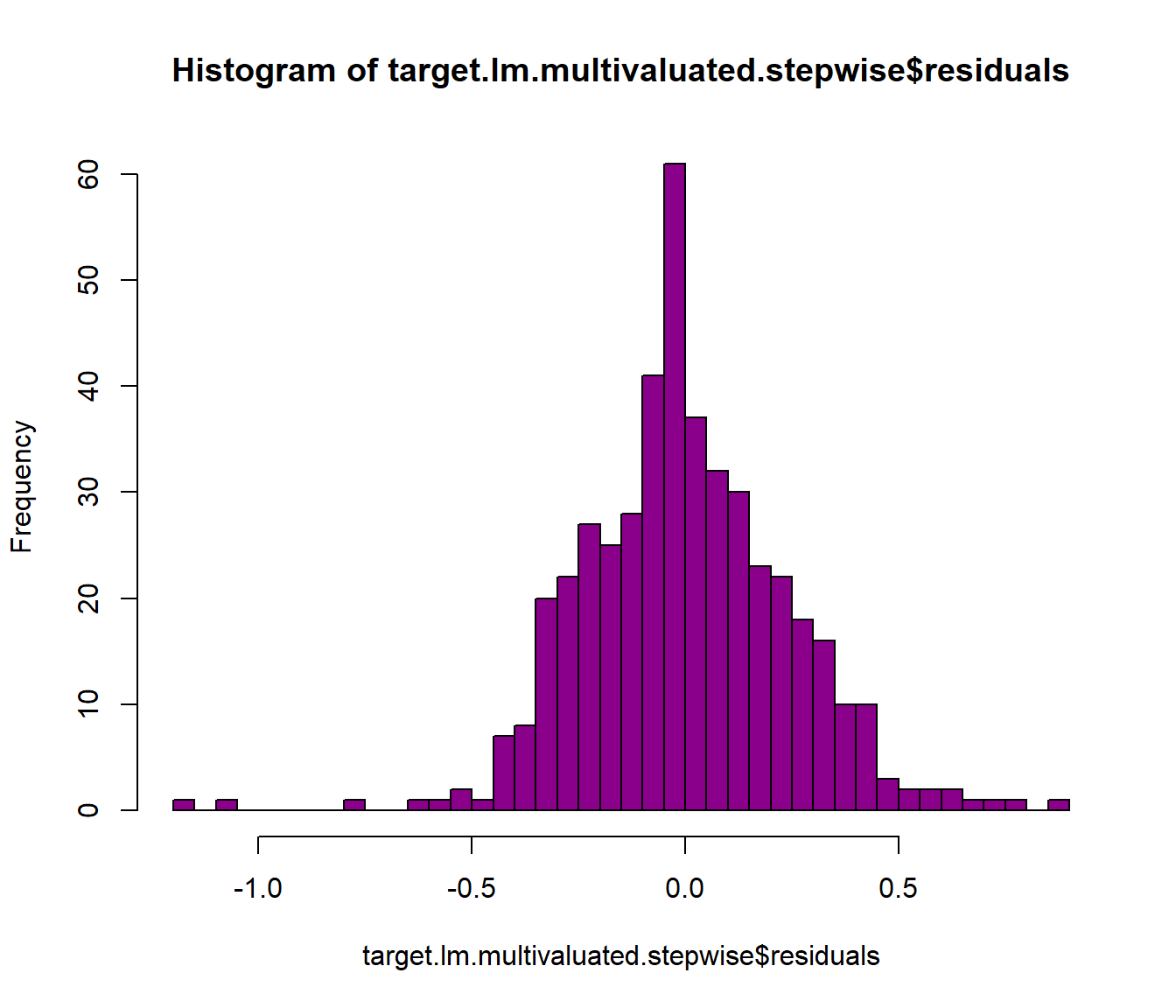
# maps
target$fitted_sem <- target.lm.multivaluated.stepwise$fitted.values
spplot(target, "fitted_sem", main = "Fitted values")
target$actual_sem <- target.lm.multivaluated.stepwise$y
spplot(target, "fitted_sem", main = "Actual values")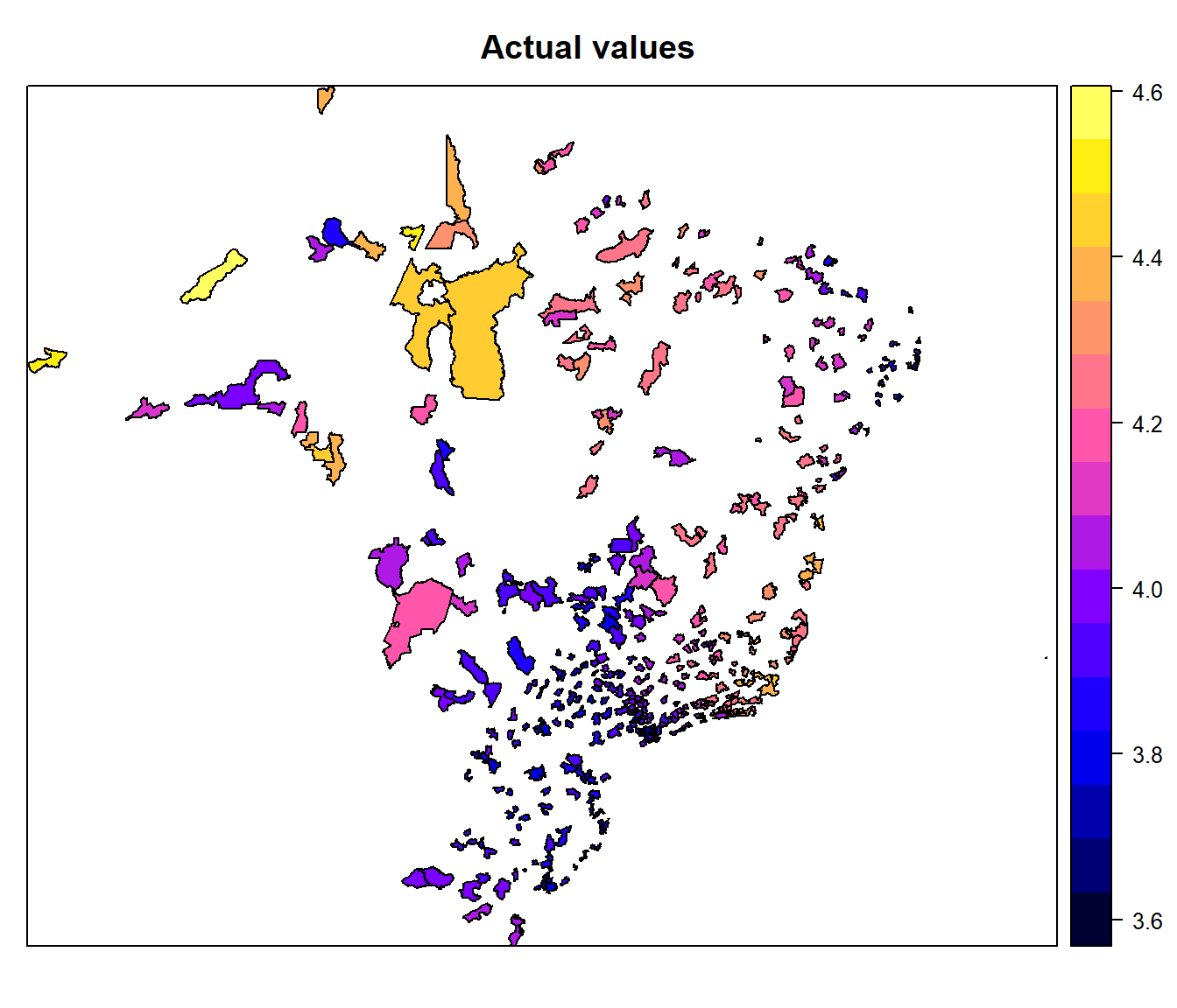
2.2 Implementando o modelo espacial auto-regressivo (SAR)
Um dos modelos mais comumente utilizados para modelagem de correlação espacial é o modelo autorregressivo espacial (do inglês spatial autorregressive model), ou simplesmente modelo SAR. A ideia dos modelos SAR é utilizar a mesma ideia dos modelos AR (autorregressivos) em séries temporais, por meio da incorporação de um termo de lag entre os regressores da equação.
Na sua forma mais simples, o modelo SAR tem expressão:
\[\gamma = \rho W \gamma + \epsilon\] Onde \(\gamma\) é um vetor coluna, contendo n observações na amostra para a variável resposta \(\gamma i\), o coeficiente escalar \(\rho\) corresponde ao parâmetro autorregressivo, esse parâmetro possui como interpretação o efeito médio da variável dependente relativo à vizinhança espacial na região em questão, já o termo \(\epsilon\) corresponde a um vetor coluna contendo os resíduos \(\epsilon i\) da equação. Por enquanto, assume-se que os resíduos \(\epsilon i\) são independentes e identicamente distribuídos, com distribuição normal, com média zero e variância homogênea \(\theta ^{2}\). Um dos componentes presentes em uma grande quantidade de modelos espaciais é a matriz \(W\). Esta matriz é conhecida como matriz de vizinhança, e pode ser definida de diversas formas, o que traz críticas aos modelos espaciais utilizando \(W\). Uma das formas mais comumente empregadas de definição da matriz \(W\) se dá por meio da identificação de vizinhos de primeira ordem.
target.sar.model <- lagsarlm(PcMedRev ~
                               DistMean +
                               DistDev +
                               DistMin +
                               RefinMean +
                               RefinDev +
                               RefinMin +
                               RefinMax +
                               ChgPIB +
                               ChgPIBCap,
                             data = target,
                             listw = lw,
                             zero.policy = T,
                             tol.solve = 1e-12)
summary(target.sar.model)
##
## Call:spatialreg::lagsarlm(formula = formula, data = data, listw = listw,
## na.action = na.action, Durbin = Durbin, type = type, method = method,
## quiet = quiet, zero.policy = zero.policy, interval = interval,
## tol.solve = tol.solve, trs = trs, control = control)
##
## Residuals:
## Min 1Q Median 3Q Max
## -1.186487 -0.154093 -0.011863 0.144570 0.877210
##
## Type: lag
## Regions with no neighbours included:
## 39255 39261 39605 39187 39223 39274 39288 39322 39378 39450 39507 39510 39515 39536 39236 39424 39572 39499 39564 39155 39179 39210 39235 39280 39283 39293 39305 39315 39337 39351 39359 39360 39373 39381 39383 39399 39416 39419 39431 39451 39454 39472 39481 39540 39551 39565 39577 39594 39225 39163 39518 39150 39197 39199 39251 39275 39297 39301 39343 39358 39363 39370 39387 39404 39410 39526 39576 39604 39376 39395 39433 39570 39585 39162 39276 39493 39209 39156 39148 39212 39232 39248 39441 39606 39169 39316 39149 39186 39189 39191 39324 39466 39483 39508 39448 39462 39469 39240 39271 39344 39385 39486 39554 39228 39418 39233 39453 39557 39176 39180 39203 39246 39300 39379 39501 39505 39548 39171 39438 39329 39375 39152 39194 39291 39327 39328 39356 39517 39546 39549 39587 39475 39484 39204 39308 39238 39256 39298 39405 39445 39452 39581 39265 39444 39516 39583 39311 39296 39397 39447 39563 39181 39365 39480
## Coefficients: (asymptotic standard errors)
## Estimate Std. Error z value Pr(>|z|)
## (Intercept) 3.8841e+00 1.1889e-01 32.6686 < 2.2e-16
## DistMean 9.4289e-04 2.6632e-04 3.5404 0.0003995
## DistDev -2.6774e-03 4.8934e-04 -5.4715 4.463e-08
## DistMin -8.2898e-04 2.9761e-04 -2.7854 0.0053455
## RefinMean -2.3316e-04 7.3625e-05 -3.1668 0.0015411
## RefinDev -1.8349e-03 1.6158e-04 -11.3561 < 2.2e-16
## RefinMin -2.8391e-04 7.5359e-05 -3.7674 0.0001650
## RefinMax 7.6570e-04 8.1385e-05 9.4083 < 2.2e-16
## ChgPIB -6.5125e+00 1.9726e+00 -3.3015 0.0009617
## ChgPIBCap 6.6688e+00 2.0050e+00 3.3260 0.0008810
##
## Rho: -0.0034761, LR test value: 0.29215, p-value: 0.58884
## Asymptotic standard error: 0.0064366
## z-value: -0.54005, p-value: 0.58916
## Wald statistic: 0.29165, p-value: 0.58916
##
## Log likelihood: -10.23669 for lag model
## ML residual variance (sigma squared): 0.061226, (sigma: 0.24744)
## Number of observations: 458
## Number of parameters estimated: 12
## AIC: 44.473, (AIC for lm: 42.766)
## LM test for residual autocorrelation
## test value: 94.639, p-value: < 2.22e-16Abaixo avaliamos os residuos e o R2 do modelo SAR.
SST <- sum((target$PcMedRev - mean(target$PcMedRev)) ^ 2)
GWR_SSE <- target.sar.model$SSE
r2_SAR <- 1 - (GWR_SSE / SST)
print(paste('R2 = ', r2_SAR))
## [1] "R2 = 0.328100732349644"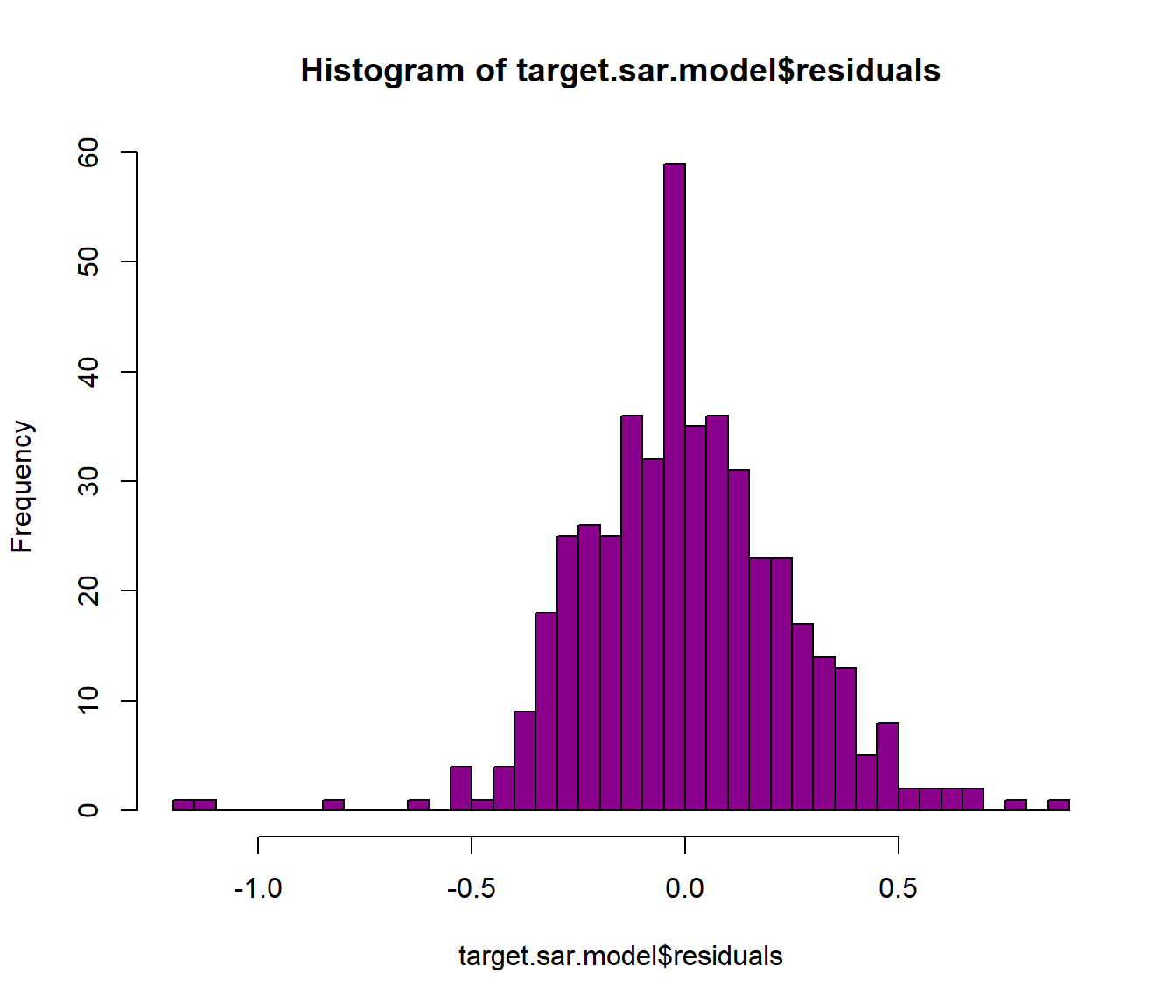
target.sar.model.residuals <- target.sar.model$residuals

target.sar.model.class_fx <- classIntervals(target.sar.model.residuals,
                                            n = 5,
                                            style = "fixed",
                                            fixedBreaks = c(-1, -.75, -.25, .25, .75, 1),
                                            rtimes = 1)

cols.sar <- findColours(target.sar.model.class_fx, pal)

plot(target, col = cols.sar, main = "SAR Model", border = "grey")
legend(x = "bottom", cex = 1, fill = attr(cols.sar, "palette"), bty = "n",
       legend = names(attr(cols.sar, "table")), title = "Residuals from SAR Model",
       ncol = 5)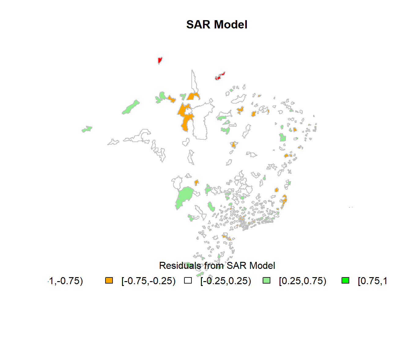
##
##  Moran I test under randomisation
##
## data:  target.sar.model.residuals
## weights: lw  n reduced by no-neighbour observations
##
##
## Moran I statistic standard deviate = 6.497, p-value = 4.098e-11
## alternative hypothesis: greater
## sample estimates:
## Moran I statistic       Expectation          Variance
##       0.414559389      -0.003300330       0.004136583
2.3 Implementando o modelo de regressão geograficamente ponderada (GWR)
O modelo GWR é um desenvolvimento de (1) para permitir a estimação dos coeficientes locais. No modelo GRW, assume-se que as informações mais próximas do ponto de regressão têm maior probabilidade de influenciá-lo.
\[\gamma_i = \beta_0(u_i, v_i) + \sum_\kappa\beta_k (u_i, v_i) \chi_i\kappa + \varepsilon_i \] Na equação, \((u_i, v_i)\) são coordenadas do ponto \(i\) no espaço (podem ser coordenadas polares, como latitudes e longitudes, por exemplo), \(\beta_0(u_i, v_i)\) é o coeficiente local estimado para o ponto \(i\).
Tal ponderação é feita pela função Kernel espacial, que é uma função real, contínua e simétrica, cuja integral soma um, semelhante a uma função de densidade de probabilidade. O Kernel espacial permite fazer a calibragem do modelo para \(n\) subamostras em torno do ponto de regressão \(i\), formando “janelas móveis”.
O modelo GWR assume que os coeficientes variem no espaço, sem uma explicação teórica fundamental. Essa variação pressupõe um determinismo geográfico que pode esconder a verdadeira causa da eventual instabilidade dos coeficientes locais. Esta observação pontua a necessidade de um olhar geral, considerando todas as demais análises realizadas durante o desenvolvimento deste projeto, para dar uma dimensão mais ampla sobre as observações que estarão presentes no relatório final (conclusão).
coords <- cbind(target$X_COORD, target$Y_COORD)

# GWR model (Geographically Weighted Regression)
target.gwr.sel <- gwr.sel(PcMedRev ~
                            DistMean +
                            DistDev +
                            DistMin +
                            RefinMean +
                            RefinDev +
                            RefinMin +
                            RefinMax +
                            ChgPIB +
                            ChgPIBCap,
                          data = target,
                          coords = coords,
                          adapt = TRUE,
                          method = "aic",
                          gweight = gwr.Gauss,
                          verbose = TRUE)
## Bandwidth: 0.381966 AIC: -17.80954
## Bandwidth: 0.618034 AIC: 10.46157
## Bandwidth: 0.236068 AIC: -50.36029
## Bandwidth: 0.145898 AIC: -77.05281
## Bandwidth: 0.09016994 AIC: -99.79467
## Bandwidth: 0.05572809 AIC: -111.5755
## Bandwidth: 0.03444185 AIC: -97.44028
## Bandwidth: 0.06347596 AIC: -108.0164
## Bandwidth: 0.04759747 AIC: -111.9414
## Bandwidth: 0.05080047 AIC: -112.3102
## Bandwidth: 0.05097047 AIC: -112.3869
## Bandwidth: 0.05278772 AIC: -112.714
## Bandwidth: 0.05253965 AIC: -112.8435
## Bandwidth: 0.05208016 AIC: -112.8153
## Bandwidth: 0.05236414 AIC: -112.9032
## Bandwidth: 0.05232345 AIC: -112.8912
## Bandwidth: 0.05240483 AIC: -112.9126
## Bandwidth: 0.05245633 AIC: -112.8863
## Bandwidth: 0.05240483 AIC: -112.9126target.gwr.model <- gwr(PcMedRev ~
DistMean +
DistDev +
DistMin +
RefinMean +
RefinDev +
RefinMin +
RefinMax +
ChgPIB +
ChgPIBCap,
data = target,
coords = coords,
bandwidth = target.gwr.sel,
gweight = gwr.Gauss,
adapt = target.gwr.sel,
hatmatrix = TRUE)Assim como para o modelo SAR avaliamos o R2 e os residuos do modelo GWR.
# calculate global residual SST (SQT)
SST <- sum((target$PcMedRev - mean(target$PcMedRev)) ^ 2)
GWR_SSE <- target.gwr.model$results$rss
r2_GWR <- 1 - (GWR_SSE / SST)
print(paste('R2 = ', r2_GWR))
## [1] "R2 = 0.658841734988261"# residuals
target.gwr.residuals <- target.gwr.model$SDF$gwr.e
hist(target.gwr.residuals, col="darkmagenta", breaks = 30)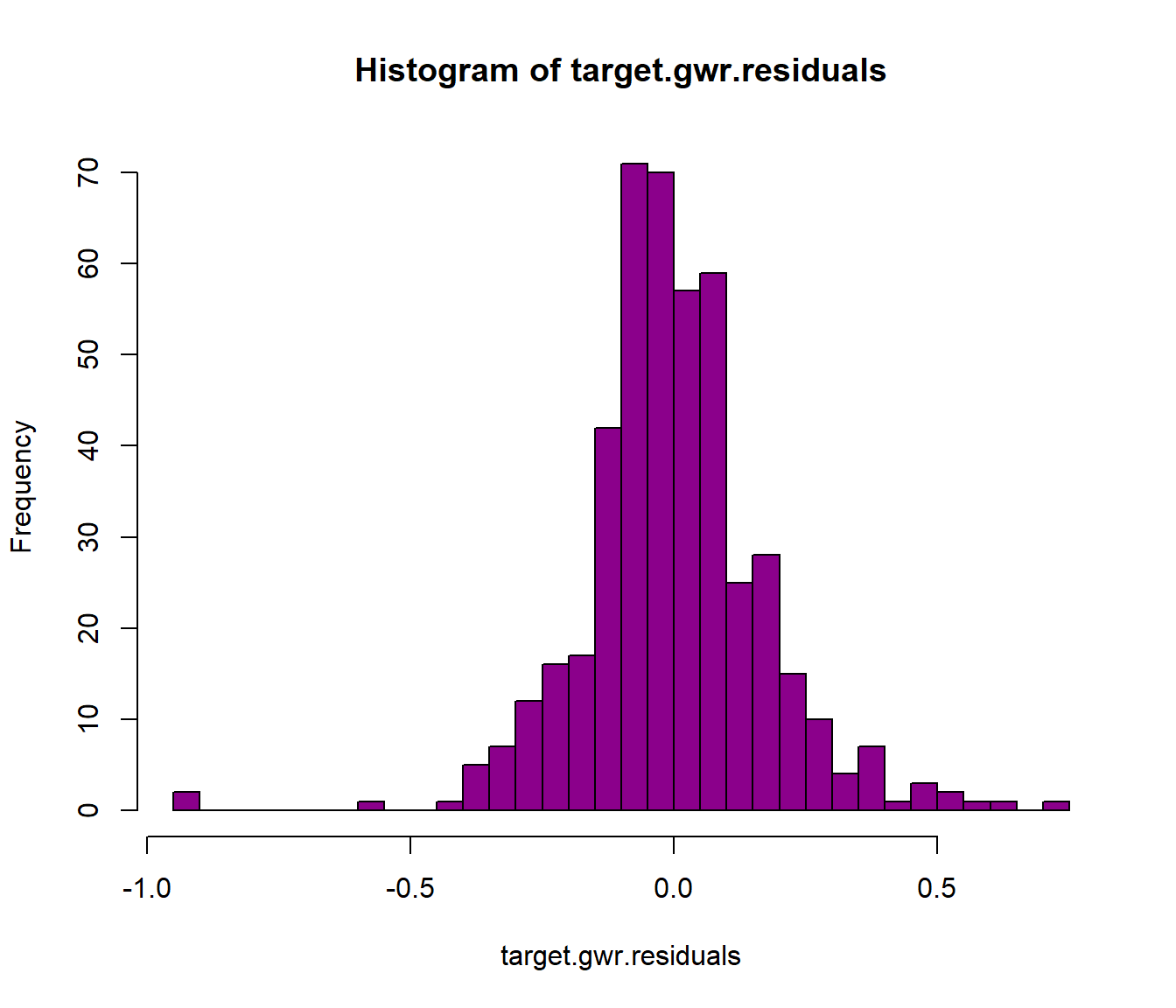
target.gwr.residuals.classes_fx <- classIntervals(target.gwr.residuals, n = 5, style = "fixed",
                                                  fixedBreaks = c(-1, -.75, -.25, .25, .75, 1),
                                                  rtimes = 1)
cols.gwr.residuals <- findColours(target.gwr.residuals.classes_fx, pal)

plot(target, col = cols.gwr.residuals, main = "GWR Model (residuals)", border = "grey")
legend(x = "bottom", cex = 1, fill = attr(cols.gwr.residuals,"palette"), bty = "n",
       legend = names(attr(cols.gwr.residuals, "table")),
       title = "Residuals from GWR Model", ncol = 5)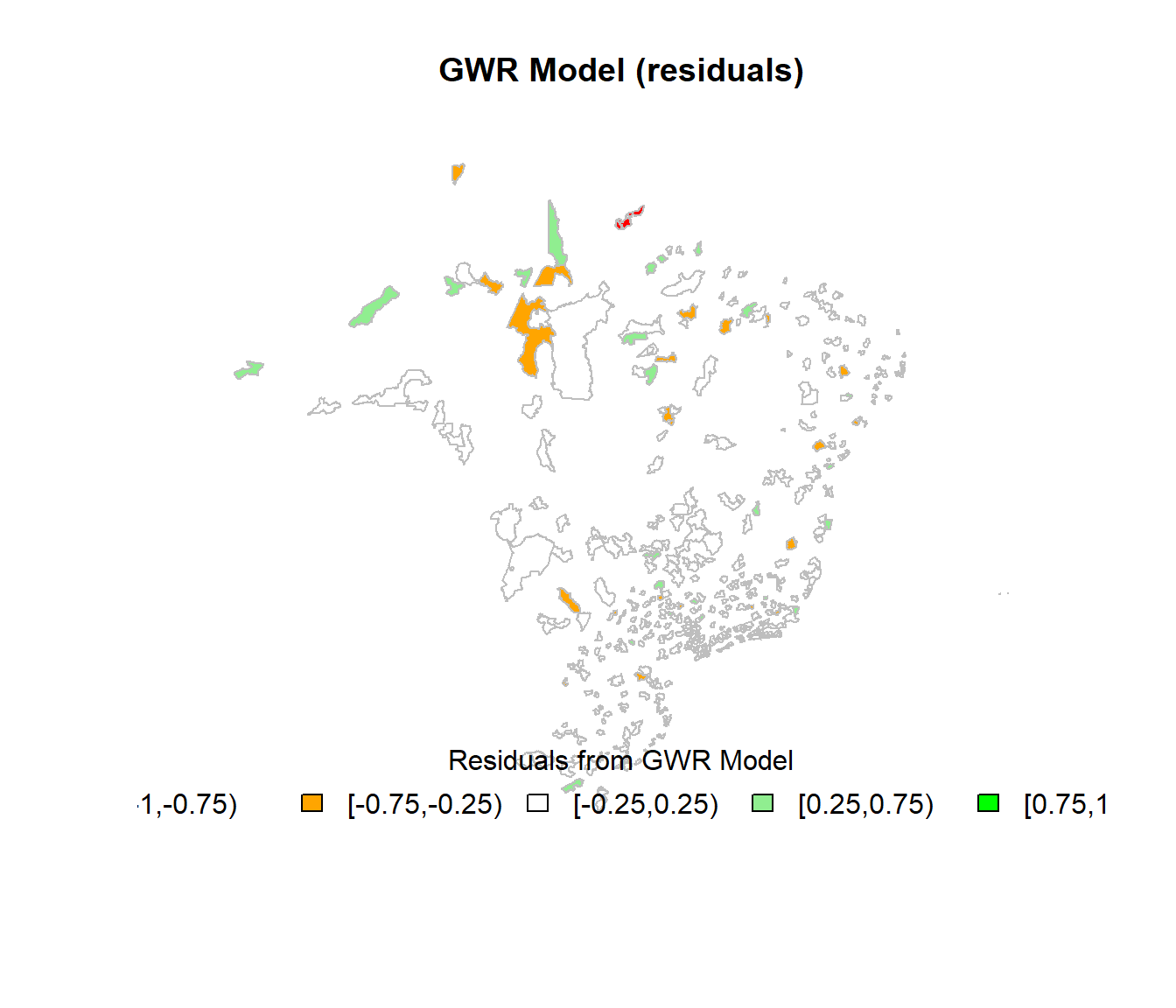
##
##  Moran I test under randomisation
##
## data:  target.gwr.residuals
## weights: lw  n reduced by no-neighbour observations
##
##
## Moran I statistic standard deviate = 2.0933, p-value = 0.01816
## alternative hypothesis: greater
## sample estimates:
## Moran I statistic       Expectation          Variance
##       0.130839530      -0.003300330       0.004106295
Finalmente para o modelo GWR podemos visualizar a dispersão geográfica dos coeficientes de uma das variáveis mais importantes do modelo, a distância média para as 10 distribuidoras mais próximas.
# coefficients
target.gwr.coefficients <- target.gwr.model$SDF$DistMean

target.gwr.coefficients.classes_fx <- classIntervals(target.gwr.coefficients, n = 5,
                                                     style = "fixed",
                                                     fixedBreaks=c(-.005,-.003,-.001,.001,.003,.005),
                                                     rtimes = 1)
cols.gwr.coefficients <- findColours(target.gwr.coefficients.classes_fx, pal)

plot(target, col = cols.gwr.coefficients, main = "GWR Model (coefficients)", border = "grey")
legend(x = "bottom", cex = 1, fill = attr(cols.gwr.coefficients,"palette"), bty = "n",
       legend = names(attr(cols.gwr.coefficients, "table")),
       title = "Local Coefficient Estimates (DistMean)", ncol = 3)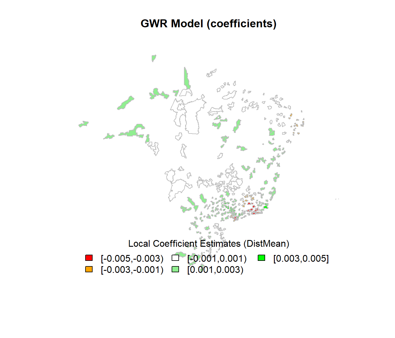
##
##  Moran I test under randomisation
##
## data:  target.gwr.coefficients
## weights: lw  n reduced by no-neighbour observations
##
##
## Moran I statistic standard deviate = 12.934, p-value < 2.2e-16
## alternative hypothesis: greater
## sample estimates:
## Moran I statistic       Expectation          Variance
##       0.824769068      -0.003300330       0.004098644