The logistic regression on loan’s report
July, 2019
1 Objective
The goal of this report is trying to fit a logistic regression model on Loan data aiming to predict the probability of delinquency for each contract.
2 Task description
2.1 Dataset preparation
Using the vanilla transaction dataset, we calculated several derived variables for each account.
First, we calculated an additional table with the current account balance and average account balance of each account.
Later on, we calculated another auxiliary table that contains the proportion of each kind of transaction (k_symbol) for each account. The idea of these variable is to capture the spend pattern of each client.
Finally, we combine the 682 Loan Contracts observations with client, district, credit card and the auxiliary tables we calculated early.
temp <- left_join(loan, disposition, by = c('account_id', 'type')) %>%
  left_join(client, by = 'client_id') %>%
  left_join(district, by = 'district_id') %>%
  left_join(creditcard, by = 'disp_id') %>%
  left_join(account_balance, by = 'account_id') %>%
  left_join(account_transaction_pattern, by = 'account_id') %>%
  mutate(card_age_month = (issued %--%
                             make_date(1998, 12, 31)) / months(1),
         last_transaction_age_days = ((last_transaction_date.y %--%
                                         make_date(1998, 12, 31)) / days(1)),
         has_card = ifelse(type.y == 'no card', 0, 1)) %>%
  dplyr::select(c("amount.x", "duration", "payments", "status", "defaulter",
                  "contract_status", "gender", "age", "district_name",
                  "region", "no_of_inhabitants",
                  "no_of_municip_inhabitants_less_499",
                  "no_of_municip_500_to_1999", "no_of_municip_2000_to_9999",
                  "no_of_municip_greater_10000", "no_of_cities",
                  "ratio_of_urban_inhabitants",
                  "average_salary", "unemploymant_rate_1995",
                  "unemploymant_rate_1996",
                  "no_of_enterpreneurs_per_1000_inhabitants",
                  "no_of_commited_crimes_1995",
                  "no_of_commited_crimes_1996", "type.y",
                  "card_age_month","account_balance",
                  "avg_balance","transaction_count", "amount.y",
                  "last_transaction_age_days", "prop_old_age_pension",
                  "prop_insurance_payment",
                  "prop_sanction_interest","prop_household",
                  "prop_statement", "prop_interest_credited",
                  "prop_loan_payment", "prop_other", "has_card"))

colnames(temp) <- c("x_loan_amount", "x_loan_duration", "x_loan_payments",
                    "x_loan_status", "y_loan_defaulter", "x_loan_contract_status",
                    "x_client_gender", "x_client_age",
                    "x_district_name", "x_region",
                    "x_no_of_inhabitants", "x_no_of_municip_inhabitants_less_499",
                    "x_no_of_municip_500_to_1999", "x_no_of_municip_2000_to_9999",
                    "x_no_of_municip_greater_10000", "x_no_of_cities",
                    "x_ratio_of_urban_inhabitants",
                    "x_average_salary", "x_unemploymant_rate_1995",
                    "x_unemploymant_rate_1996",
                    "x_no_of_enterpreneurs_per_1000_inhabitants",
                    "x_no_of_commited_crimes_1995",
                    "x_no_of_commited_crimes_1996", "x_card_type",
                    "x_card_age_month","x_account_balance",
                    "x_avg_account_balance","x_transaction_count",
                    "x_transaction_amount", "x_last_transaction_age_days",
                    "x_prop_old_age_pension", "x_prop_insurance_payment",
                    "x_prop_sanction_interest","x_prop_household","x_prop_statement",
                    "x_prop_interest_credited", "x_prop_loan_payment", "x_prop_other",
                    "x_has_card")

temp <- dplyr::select(temp, y_loan_defaulter, everything())

temp$x_card_type = ifelse(is.na(temp$x_card_type), 'no card',
                          as.character(temp$x_card_type))

temp$x_has_card = ifelse(temp$x_card_type == 'no card', 0, 1)

temp$x_card_age_month = ifelse(is.na(temp$x_card_age_month), 0,
                               temp$x_card_age_month)

temp$y_loan_defaulter = as.numeric(temp$y_loan_defaulter)
We ended up having a data set with 39 variables.
| variables |
|---|
| y_loan_defaulter |
| x_loan_amount |
| x_loan_duration |
| x_loan_payments |
| x_loan_status |
| x_loan_contract_status |
| x_client_gender |
| x_client_age |
| x_district_name |
| x_region |
| x_no_of_inhabitants |
| x_no_of_municip_inhabitants_less_499 |
| x_no_of_municip_500_to_1999 |
| x_no_of_municip_2000_to_9999 |
| x_no_of_municip_greater_10000 |
| x_no_of_cities |
| x_ratio_of_urban_inhabitants |
| x_average_salary |
| x_unemploymant_rate_1995 |
| x_unemploymant_rate_1996 |
| x_no_of_enterpreneurs_per_1000_inhabitants |
| x_no_of_commited_crimes_1995 |
| x_no_of_commited_crimes_1996 |
| x_card_type |
| x_card_age_month |
| x_account_balance |
| x_avg_account_balance |
| x_transaction_count |
| x_transaction_amount |
| x_last_transaction_age_days |
| x_prop_old_age_pension |
| x_prop_insurance_payment |
| x_prop_sanction_interest |
| x_prop_household |
| x_prop_statement |
| x_prop_interest_credited |
| x_prop_loan_payment |
| x_prop_other |
| x_has_card |
2.2 Variable selection
From this dataset, we excluded 6 variables that are redundant, shows no variability on the 682 Loan contract observations or have no applicability for the exercise:
- x_prop_old_age_pension (no variation on selected sample);
- x_district_name (sample have not enough variability to fit a model);
- x_region (sample have not enough variability to fit a model);
- x_loan_status (redundant);
- x_loan_contract_status (redundant);
- x_prop_sanction_interest (seems not to be valid for this analysis, as the reason for interest payment in the account is exactly the delinquency in the observation contact itself).
2.3 Investigating Multicollinearity
With the remaining variables we ran a multicollinearity test to identify additional variables to drop from the model specification.
vars.quant <- select_if(temp, is.numeric)
VIF <- imcdiag(vars.quant, temp$y_loan_defaulter)

VIF_Table_Before <- tibble(variable = names(VIF$idiags[,1]),
                    VIF = VIF$idiags[,1]) %>%
             arrange(desc(VIF))

kable(VIF_Table_Before)| variable | VIF |
|---|---|
| x_no_of_inhabitants | 161.078688 |
| x_prop_other | 156.614374 |
| x_no_of_commited_crimes_1996 | 153.788642 |
| x_prop_household | 119.766648 |
| x_prop_interest_credited | 62.164451 |
| x_prop_loan_payment | 42.215533 |
| x_prop_insurance_payment | 33.065760 |
| x_transaction_amount | 13.077575 |
| x_prop_statement | 12.611010 |
| x_transaction_count | 12.243487 |
| x_unemploymant_rate_1996 | 11.942010 |
| x_unemploymant_rate_1995 | 11.457609 |
| x_average_salary | 10.592530 |
| x_no_of_cities | 5.348665 |
| x_no_of_enterpreneurs_per_1000_inhabitants | 4.398114 |
| x_no_of_municip_2000_to_9999 | 4.342691 |
| x_ratio_of_urban_inhabitants | 4.141633 |
| x_loan_amount | 3.656975 |
| x_no_of_municip_500_to_1999 | 3.494354 |
| x_loan_payments | 3.467355 |
| x_no_of_commited_crimes_1995 | 3.343160 |
| x_no_of_municip_greater_10000 | 2.784531 |
| x_loan_duration | 2.634738 |
| x_has_card | 2.365295 |
| x_no_of_municip_inhabitants_less_499 | 2.353720 |
| x_card_age_month | 2.200021 |
| x_avg_account_balance | 1.842499 |
| y_loan_defaulter | 1.728511 |
| x_account_balance | 1.422176 |
| x_last_transaction_age_days | 1.068578 |
| x_client_age | 1.053711 |
ggplot(VIF_Table_Before, aes(x = fct_reorder(variable, VIF), y = log(VIF), label = round(VIF, 2))) +
  geom_point(stat='identity', fill="black", size=15)  +
  geom_segment(aes(y = 0,
                   yend = log(VIF),
                   xend = variable),
               color = "black") +
  geom_text(color="white", size=4) +
  geom_hline(aes(yintercept = log(5)), color = 'red', size = 2) +
  scale_y_continuous(labels = NULL, breaks = NULL) +
  coord_flip() +
  theme_economist() +
  theme(legend.position = 'none',
        panel.grid.major = element_blank(),
        panel.grid.minor = element_blank()) +
  labs(x = 'Variable',
       y = NULL,
       title = 'Variance Inflation Factor',
       subtitle="Checking for multicolinearity in X's variables.
       Variables with VIF more than 5 will
       be droped from the model")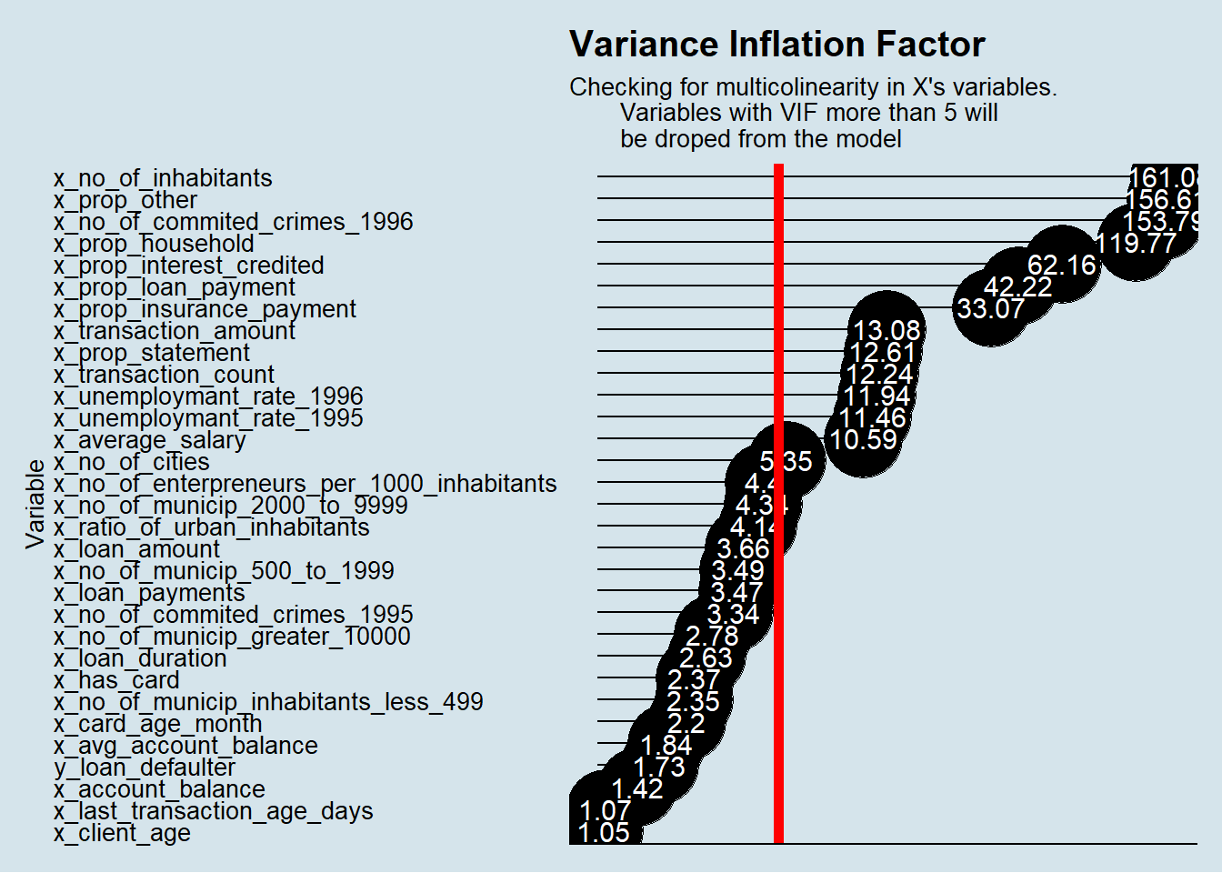
We decided to exclude any variable with a VIF greater than 5.
Below variables were excluded based on the multicollinear presence on them.
- x_prop_insurance_payment;
- x_prop_household;
- x_prop_statement ;
- x_prop_loan_payment;
- x_prop_other;
- x_no_of_inhabitants;
- x_no_of_commited_crimes_1996;
- x_transaction_amount;
- x_transaction_count;
- x_unemploymant_rate_1996;
- x_unemploymant_rate_1995;
- x_average_salary;
- x_no_of_cities.
temp <- dplyr::select(temp, -c(x_prop_insurance_payment,
                               x_prop_household,
                               x_prop_statement,
                               x_prop_loan_payment,
                               x_prop_other,
                               x_no_of_inhabitants,
                               x_no_of_commited_crimes_1996,
                               x_transaction_amount,
                               x_transaction_count,
                               x_unemploymant_rate_1996,
                               x_unemploymant_rate_1995,
                               x_average_salary,
                               x_no_of_cities))

loan_reg_dataset <- temp
Here is the final correlation matrix we got:
| variable | VIF |
|---|---|
| x_loan_amount | 3.576281 |
| x_no_of_municip_500_to_1999 | 2.781569 |
| x_no_of_municip_2000_to_9999 | 2.565167 |
| x_loan_duration | 2.366083 |
| x_no_of_enterpreneurs_per_1000_inhabitants | 2.289033 |
| x_has_card | 2.242915 |
| x_loan_payments | 2.208547 |
| x_no_of_municip_greater_10000 | 2.147182 |
| x_card_age_month | 2.028568 |
| x_ratio_of_urban_inhabitants | 1.986178 |
| x_no_of_municip_inhabitants_less_499 | 1.881482 |
| x_no_of_commited_crimes_1995 | 1.798576 |
| x_avg_account_balance | 1.656011 |
| x_account_balance | 1.378326 |
| x_prop_interest_credited | 1.280158 |
| y_loan_defaulter | 1.242373 |
| x_last_transaction_age_days | 1.048220 |
| x_client_age | 1.040390 |
Plot of VIF values:
ggplot(VIF_Table_After, aes(x = fct_reorder(variable, VIF), y = log(VIF), label = round(VIF, 2))) +
  geom_point(stat='identity', fill="black", size=15)  +
  geom_segment(aes(y = 0,
                   yend = log(VIF),
                   xend = variable),
               color = "black") +
  geom_text(color="white", size=4) +
  geom_hline(aes(yintercept = log(5)), color = 'red', size = 2) +
  scale_y_continuous(labels = NULL, breaks = NULL) +
  coord_flip() +
  theme_economist() +
  theme(legend.position = 'none',
        panel.grid.major = element_blank(),
        panel.grid.minor = element_blank()) +
  labs(x = 'Variable',
       y = NULL,
       title = 'Variance Inflation Factor',
       subtitle="Checking for multicolinearity in X's variables.
       Variables with VIF more than 5 will
       be droped from the model")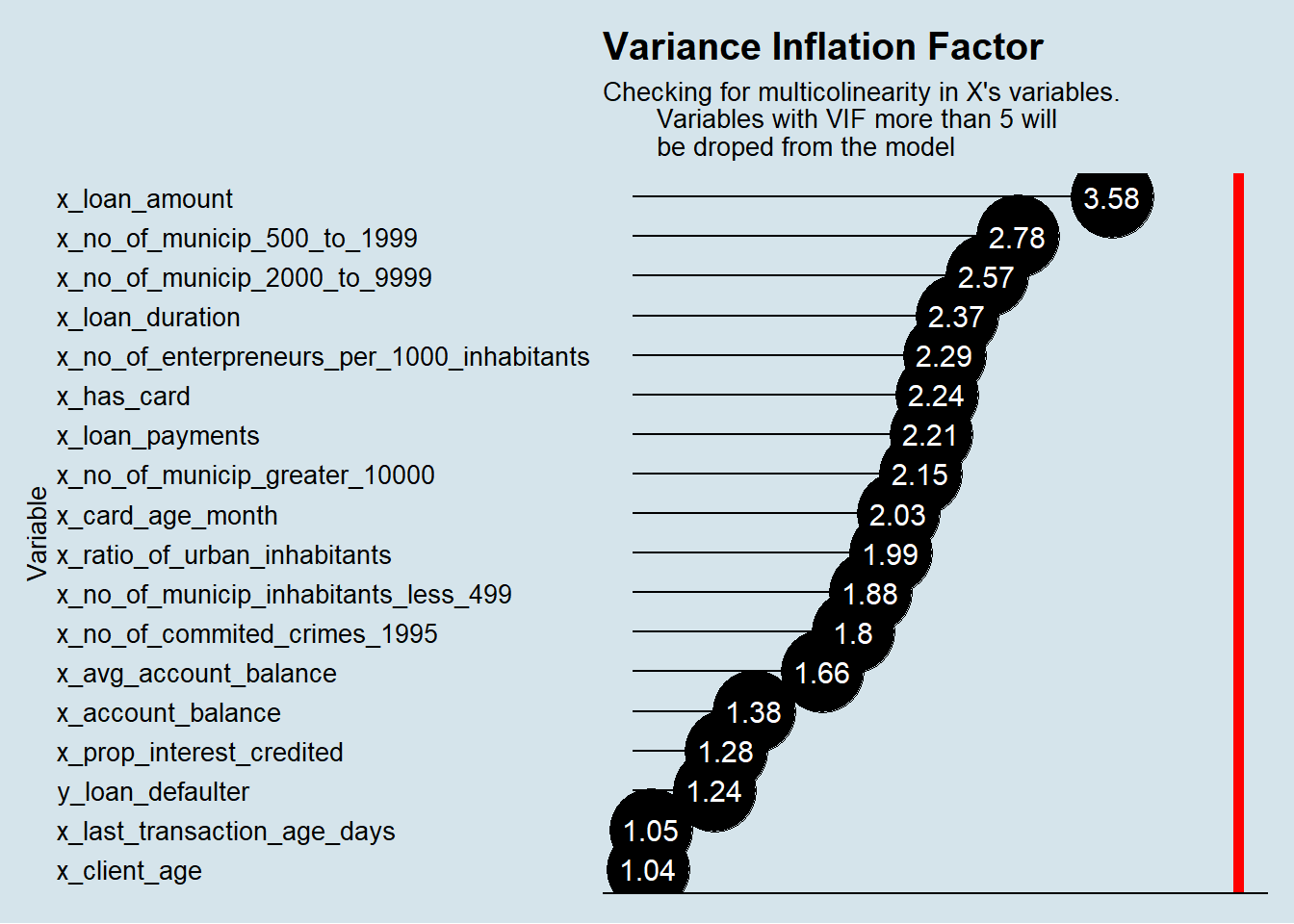
Correlation Matrix Plot: no Variable with correlation more than 0.6.
cor_mtx <- cor(vars.quant)

ggcorrplot(cor_mtx, hc.order = TRUE,
           type = "lower",
           lab = TRUE,
           lab_size = 3,
           method="circle",
           colors = c("tomato2", "white", "springgreen3"),
           title="Correlation Matrix of Loan Dataset",
           ggtheme=theme_bw)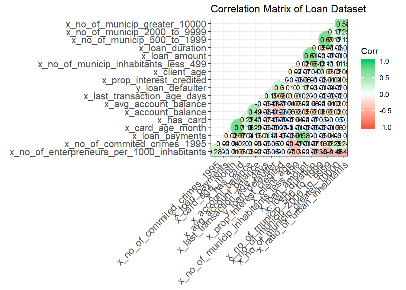
2.4 Sample split into Test and Training Data
The available data in Loan Dataset is split into Train and Testing data on the following proportion:
- Train Dataset (70% 478 obs);
- Test Dataset (30% 204 obs).
set.seed(12345)
index <- caret::createDataPartition(loan_reg_dataset$y_loan_defaulter,
                                    p= 0.7,list = FALSE)

data.train <- loan_reg_dataset[index, ]
data.test  <- loan_reg_dataset[-index,]


event_proportion <- bind_rows(prop.table(table(loan_reg_dataset$y_loan_defaulter)),
                              prop.table(table(data.train$y_loan_defaulter)),
                              prop.table(table(data.test$y_loan_defaulter)))

event_proportion$scope = ''
event_proportion$scope[1] = 'full dataset'
event_proportion$scope[2] = 'train dataset'
event_proportion$scope[3] = 'test dataset'

event_proportion <- select(event_proportion, scope, everything())

kable(event_proportion)| scope | 0 | 1 |
|---|---|---|
| full dataset | 0.8885630 | 0.1114370 |
| train dataset | 0.8933054 | 0.1066946 |
| test dataset | 0.8774510 | 0.1225490 |
Both datasets keep the same proportion for the explained variable around 11%.
2.5 Fit the logistic model
With the final cleaned dataset, we got from above steps we fit our Logistic Regression Y_loan_defaulter on all x variables.
model_1 <- glm(data = data.train, formula = y_loan_defaulter ~ .,
                 family= binomial(link='logit'))

# jut truncating variable names to 30 char to fit nicely in the screen.
names(model_1$coefficients) <- stringr::str_sub(names(model_1$coefficients), 1, 30)

summary(model_1)
##
## Call:
## glm(formula = y_loan_defaulter ~ ., family = binomial(link = "logit"),
## data = data.train)
##
## Deviance Residuals:
## Min 1Q Median 3Q Max
## -1.5308 -0.4369 -0.2692 -0.1609 2.9273
##
## Coefficients: (1 not defined because of singularities)
## Estimate Std. Error z value Pr(>|z|)
## (Intercept) -4.405e+00 2.351e+00 -1.874 0.0610 .
## x_loan_amount 7.239e-06 2.978e-06 2.431 0.0151 *
## x_loan_duration -2.860e-02 1.867e-02 -1.532 0.1255
## x_loan_payments 2.306e-03 1.839e-03 1.254 0.2099
## x_client_gendermale 2.084e-02 3.594e-01 0.058 0.9537
## x_client_age 1.801e-02 1.414e-02 1.274 0.2028
## x_no_of_municip_inhabitants_le -1.823e-03 6.599e-03 -0.276 0.7824
## x_no_of_municip_500_to_1999 8.119e-04 1.957e-02 0.041 0.9669
## x_no_of_municip_2000_to_9999 -1.178e-02 6.436e-02 -0.183 0.8547
## x_no_of_municip_greater_10000 -3.642e-01 2.321e-01 -1.569 0.1167
## x_ratio_of_urban_inhabitants 9.512e-03 1.150e-02 0.827 0.4080
## x_no_of_enterpreneurs_per_1000 -1.078e-02 1.162e-02 -0.927 0.3538
## x_no_of_commited_crimes_1995 -1.362e-02 9.617e-03 -1.416 0.1566
## x_card_typegold 5.329e-01 1.315e+00 0.405 0.6852
## x_card_typejunior 3.728e-01 1.311e+00 0.284 0.7762
## x_card_typeno card 1.580e+00 8.938e-01 1.768 0.0770 .
## x_card_age_month 2.938e-02 3.072e-02 0.956 0.3390
## x_account_balance 2.386e-06 1.383e-06 1.725 0.0844 .
## x_avg_account_balance -4.174e-06 2.969e-06 -1.406 0.1598
## x_last_transaction_age_days 2.641e-02 4.276e-02 0.618 0.5368
## x_prop_interest_credited 1.156e+01 2.241e+00 5.158 2.5e-07 ***
## x_has_card NA NA NA NA
## ---
## Signif. codes: 0 '***' 0.001 '**' 0.01 '*' 0.05 '.' 0.1 ' ' 1
##
## (Dispersion parameter for binomial family taken to be 1)
##
## Null deviance: 324.61 on 477 degrees of freedom
## Residual deviance: 246.59 on 457 degrees of freedom
## AIC: 288.59
##
## Number of Fisher Scoring iterations: 6Alternatively we fit a second model only with variables statistically significant p-value less than 10%.
model_2 <- glm(data = data.train, formula = y_loan_defaulter ~ x_loan_amount +
                 x_loan_duration + x_has_card + x_prop_interest_credited,
                 family= binomial(link='logit'))

# jut truncating variable names to 30 char to fit nicely in the screen.
names(model_2$coefficients) <- stringr::str_sub(names(model_2$coefficients), 1, 30)

summary(model_2)
##
## Call:
## glm(formula = y_loan_defaulter ~ x_loan_amount + x_loan_duration +
## x_has_card + x_prop_interest_credited, family = binomial(link = "logit"),
## data = data.train)
##
## Deviance Residuals:
## Min 1Q Median 3Q Max
## -1.5790 -0.4375 -0.3290 -0.2165 2.6686
##
## Coefficients:
## Estimate Std. Error z value Pr(>|z|)
## (Intercept) -3.632e+00 4.984e-01 -7.286 3.19e-13 ***
## x_loan_amount 9.023e-06 1.888e-06 4.780 1.75e-06 ***
## x_loan_duration -3.864e-02 1.458e-02 -2.651 0.00803 **
## x_has_card -1.064e+00 5.009e-01 -2.124 0.03364 *
## x_prop_interest_credited 9.715e+00 1.750e+00 5.551 2.85e-08 ***
## ---
## Signif. codes: 0 '***' 0.001 '**' 0.01 '*' 0.05 '.' 0.1 ' ' 1
##
## (Dispersion parameter for binomial family taken to be 1)
##
## Null deviance: 324.61 on 477 degrees of freedom
## Residual deviance: 264.00 on 473 degrees of freedom
## AIC: 274
##
## Number of Fisher Scoring iterations: 6In the next step we will compare how each model performed.
3 Evaluating the model performance
We started this step by making predictions using our model on the X’s variables in our Train and Test datasets.
glm.prob.train.1 <- predict(model_1, type = "response")
glm.prob.test.1 <- predict(model_1, newdata = data.test, type= "response")

glm.prob.train.2 <- predict(model_2, type = "response")
glm.prob.test.2 <- predict(model_2, newdata = data.test, type= "response")
We then evaluate the metrics in the each model for Train and Test data:
glm.train.1 <- HMeasure(data.train$y_loan_defaulter, glm.prob.train.1, threshold = 0.5)
glm.test.1  <- HMeasure(data.test$y_loan_defaulter, glm.prob.test.1, threshold = 0.5)

glm.train.2 <- HMeasure(data.train$y_loan_defaulter, glm.prob.train.2, threshold = 0.5)
glm.test.2 <- HMeasure(data.test$y_loan_defaulter, glm.prob.test.2, threshold = 0.5)

measures <- t(bind_rows(glm.train.1$metrics,
                      glm.test.1$metrics,
                      glm.train.2$metrics,
                      glm.test.2$metrics)) %>% as_tibble(., rownames = NA)

colnames(measures) <- c('model 1 - train','model 1 - test',
                        'model 2 - train','model 2 - test')

measures$metric = rownames(measures)

measures <- select(measures, metric, everything())

kable(measures, row.names = FALSE)| metric | model 1 - train | model 1 - test | model 2 - train | model 2 - test |
|---|---|---|---|---|
| H | 0.3782094 | 0.3436917 | 0.3259694 | 0.4267060 |
| Gini | 0.6830601 | 0.5642458 | 0.6040777 | 0.6420112 |
| AUC | 0.8415301 | 0.7821229 | 0.8020388 | 0.8210056 |
| AUCH | 0.8567066 | 0.8179888 | 0.8227029 | 0.8521788 |
| KS | 0.5430959 | 0.4563128 | 0.5100335 | 0.5450279 |
| MER | 0.0962343 | 0.0980392 | 0.0941423 | 0.1078431 |
| MWL | 0.0870958 | 0.1169262 | 0.0933982 | 0.0978470 |
| Spec.Sens95 | 0.5035129 | 0.3016760 | 0.3161593 | 0.3743017 |
| Sens.Spec95 | 0.3921569 | 0.4000000 | 0.3333333 | 0.4000000 |
| ER | 0.1025105 | 0.1176471 | 0.0983264 | 0.1176471 |
| Sens | 0.1764706 | 0.1600000 | 0.1568627 | 0.1600000 |
| Spec | 0.9836066 | 0.9832402 | 0.9906323 | 0.9832402 |
| Precision | 0.5625000 | 0.5714286 | 0.6666667 | 0.5714286 |
| Recall | 0.1764706 | 0.1600000 | 0.1568627 | 0.1600000 |
| TPR | 0.1764706 | 0.1600000 | 0.1568627 | 0.1600000 |
| FPR | 0.0163934 | 0.0167598 | 0.0093677 | 0.0167598 |
| F | 0.2686567 | 0.2500000 | 0.2539683 | 0.2500000 |
| Youden | 0.1600771 | 0.1432402 | 0.1474951 | 0.1432402 |
| TP | 9.0000000 | 4.0000000 | 8.0000000 | 4.0000000 |
| FP | 7.0000000 | 3.0000000 | 4.0000000 | 3.0000000 |
| TN | 420.0000000 | 176.0000000 | 423.0000000 | 176.0000000 |
| FN | 42.0000000 | 21.0000000 | 43.0000000 | 21.0000000 |
Then, we look a boxplot chart to see how well our model split the observation into our explained variable:
-Model 1: 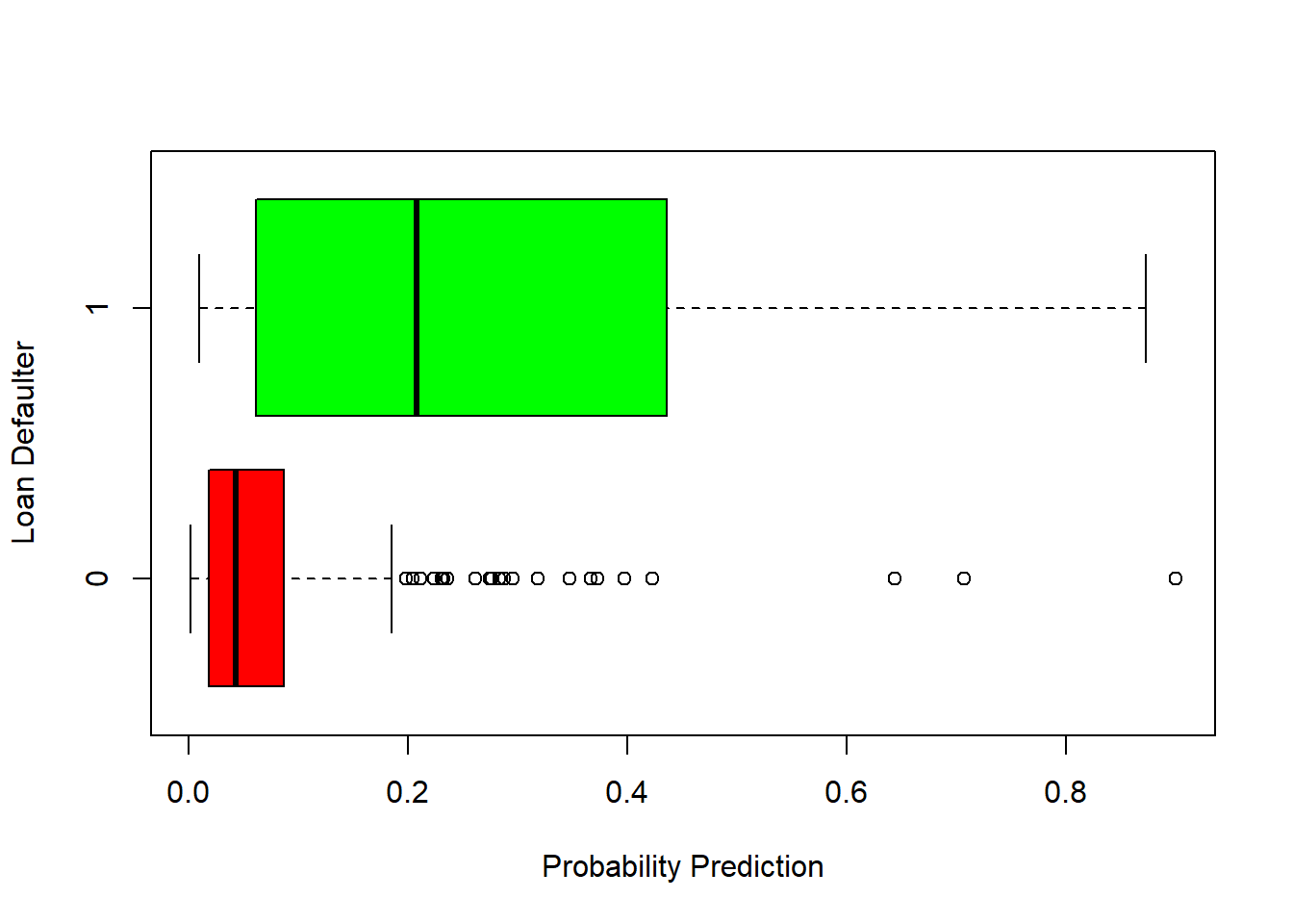
-Model 2: 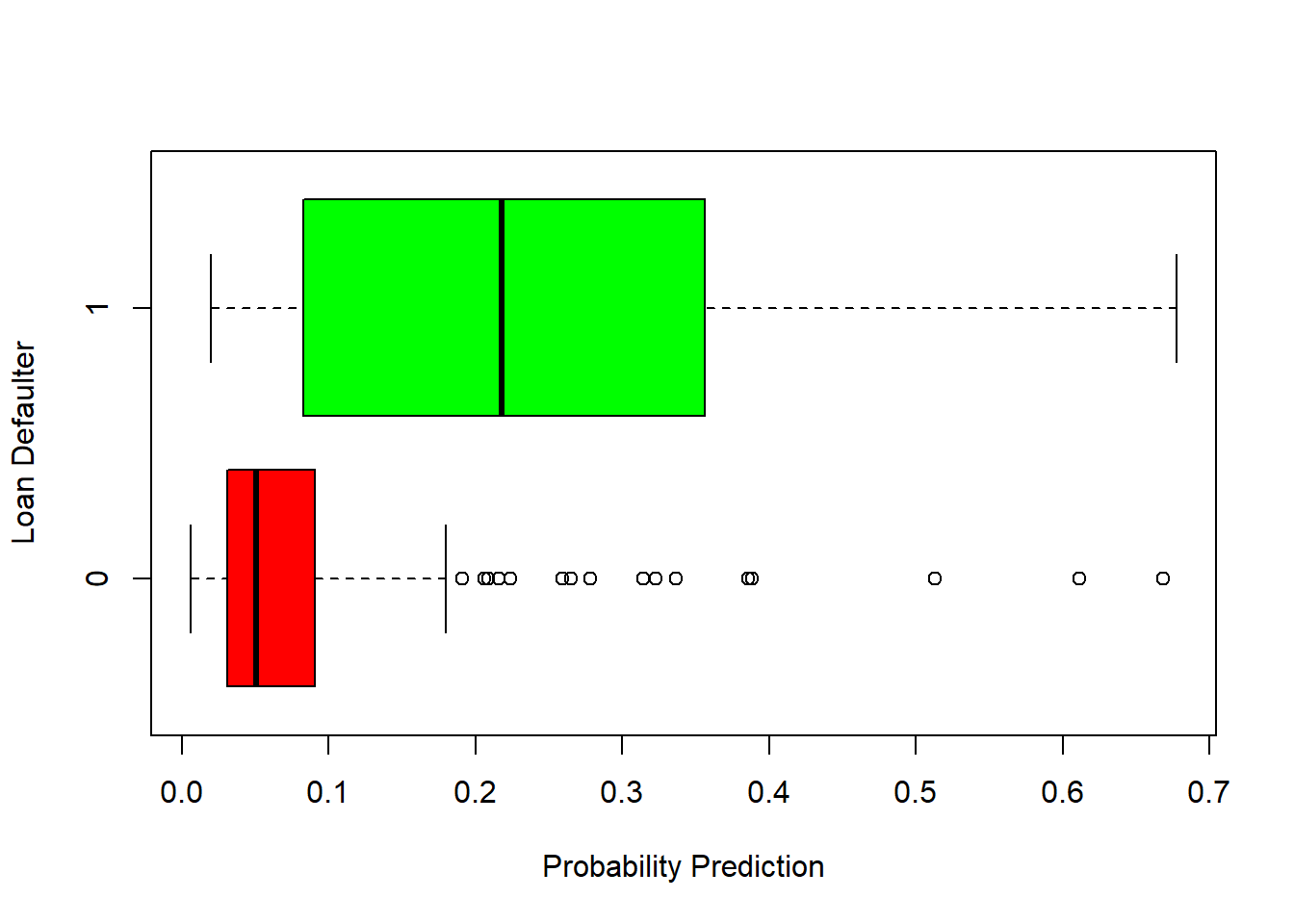
Then we plot the ROC(Receiver Operator Characteristic Curve) of the model:
roc_1 <- roc(data.test$y_loan_defaulter, glm.prob.test.1)
roc_2 <- roc(data.test$y_loan_defaulter, glm.prob.test.2)

y1 <- roc_1$sensitivities
x1 <- 1-roc_1$specificities

y2 <- roc_2$sensitivities
x2 <- 1-roc_2$specificities

plot(x1, y1,  type="n",
     xlab = "False Positive Rate (Specificities)",
     ylab= "True Positive Rate (Sensitivities)")

lines(x1, y1,lwd=3,lty=1, col="red")
lines(x2, y2,lwd=3,lty=1, col="blue")

abline(0,1, lty=2)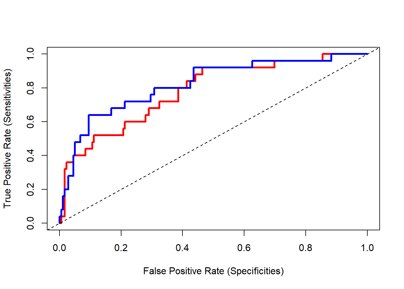
By the ROC curve of each model we see that model 2 is a better model. It only consider the statistic significant variables.
Finally we look more closely to the model 2 accuracy:
-Model 2:
To perform this task, we start by defining a threshold to assign the observation to each class, and them calculate the General Accuracy and the True Positive Rate. We start our analysis with a threshold of 0.5
threshold <- 0.5

fitted.results.2 <- ifelse(glm.prob.test.2 > threshold ,1 ,0)

misClasificError <- mean(fitted.results.2 != data.test$y_loan_defaulter)

misClassCount <- misclassCounts(fitted.results.2, data.test$y_loan_defaulter)

paste('Model General Accuracy of: ', round((1 - misClassCount$metrics['ER']) * 100, 2), '%', sep = '')
## [1] "Model General Accuracy of: 88.24%"## [1] "True Positive Rate of : 16%"| pred.1 | pred.0 | |
|---|---|---|
| actual.1 | 4 | 21 |
| actual.0 | 3 | 176 |
At a first glance we may see this model as an excellent predictor of default as it can predict the correct class 88.24% of the cases.
But looking more closely at the confusion matrix we can see that this model can predict only 16% of the true defaulters.
One way to improve the performance of the model is to decrease the threshold to 0.2.
See results below:
threshold <- 0.2

fitted.results.2 <- ifelse(glm.prob.test.2 > threshold ,1 ,0)

misClasificError <- mean(fitted.results.2 != data.test$y_loan_defaulter)

misClassCount <- misclassCounts(fitted.results.2, data.test$y_loan_defaulter)

paste('Model General Accuracy of: ', round((1 - misClassCount$metrics['ER']) * 100, 2), '%', sep = '')
## [1] "Model General Accuracy of: 86.76%"## [1] "True Positive Rate of : 52%"| pred.1 | pred.0 | |
|---|---|---|
| actual.1 | 13 | 12 |
| actual.0 | 15 | 164 |
Now we see that the True Positive accuracy increased to 52% and the general accuracy drop just a bit to 86.76%.
We may be tempted to reduce even more our threshold.
Let’s see what happen if we use 0.1 as threshold.
## [1] "Model General Accuracy of: 76.47%"## [1] "True Positive Rate of : 72%"| pred.1 | pred.0 | |
|---|---|---|
| actual.1 | 18 | 7 |
| actual.0 | 41 | 138 |
Now our TPR jumped to 72% and our general accuracy drop to 76.47%.
The final threshold will depend on the real word use case, by how much we value each class.
In this sample we see that we can improve our True Positive prediction rate at expense of classifying an increasing number as defaulter.
This balance must be decided by the managers and the bank should keep seeking and experimenting with more variables to find a better model.